

A Poisson process, or Poisson point process, describes a process where certain events occur at a constant rate, but at random and independently of each other. A poisson distribution is a discrete probability distribution that measures the probability of a certain number of events occurring within a specified period of time, given that these events occur at a constant average rate and independently of the previous event.
What Is a Poisson Distribution and a Poisson Process?
A Poisson distribution model helps find the probability of a given number of events in a time period, or the probability of waiting time until the next event in a Poisson process (where certain events occur randomly and independently but at a continuous rate).
Let’s look at Poisson processes and the Poisson distribution, two important probability concepts in statistics. After highlighting the relevant theory, we’ll work through a real-world example.
What Is a Poisson Process?
A Poisson process is a model for a series of discrete events where the average time between events is known, but the exact timing of events is random. The arrival of an event is independent of the event before (waiting time between events is memoryless). For example, suppose we own a website that our content delivery network (CDN) tells us goes down on average once per 60 days, but one failure doesn’t affect the probability of the next. All we know is the average time between failures. The failures are a Poisson process that looks like:
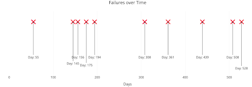
We know the average time between events, but the events are randomly spaced in time (stochastic). We might have back-to-back failures, but we could also go years between failures because the process is stochastic.
A Poisson process meets the following criteria (in reality, many phenomena modeled as Poisson processes don’t precisely match these but can be approximated as such):
Poisson Process Criteria
- Events are independent of each other. The occurrence of one event does not affect the probability another event will occur.
- The average rate (events per time period) is constant.
- Two events cannot occur at the same time.
The last point — events are not simultaneous — means we can think of each sub-interval in a Poisson process as a Bernoulli Trial, that is, either a success or a failure. With our website, the entire interval in consideration is 60 days, but each with sub-interval (one day) our website either goes down or it doesn’t.
Common examples of Poisson processes are customers calling a help center, visitors to a website, radioactive decay in atoms, photons arriving at a space telescope and movements in a stock price. Poisson processes are generally associated with time, but they don’t have to be. In the case of stock prices, we might know the average movements per day (events per time), but we could also have a Poisson process for the number of trees in an acre (events per area).
One example of a Poisson process we often see is bus arrivals (or trains). However, this isn’t a proper Poisson process because the arrivals aren’t independent of one another. Even for bus systems that run on time, a late arrival from one bus can impact the next bus’s arrival time. Jake VanderPlas has a great article on applying a Poisson process to bus arrival times which works better with made-up data than real-world data.
What Is a Poisson Distribution?
The Poisson distribution and its formula helps find the probability of a given number of events in a time period, or find the probability of waiting some time until the next event. As a Poisson process is a model we use for describing randomly occurring events (which by itself isn’t that useful), Poisson distribution helps to make sense of the Poisson process model.
The Poisson distribution probability mass function (pmf) gives the probability of observing k events in a time period given the length of the period and the average events per time.
We can use the Poisson distribution pmf to find the probability of observing a number of events over an interval generated by a Poisson process. Another use of the mass function equation (as we’ll see later) is to find the probability of waiting a given amount of time between events.
Poisson Distribution Formula
The Poisson distribution formula, which helps determine the pmf, is as follows:

The pmf is a little convoluted, and we can simplify events/time * time period into a single parameter, lambda (λ), the rate parameter. With this substitution, the Poisson Distribution probability function now has one parameter:

In a Poisson distribution formula:
- k is the number of events that occurred in a given time period or interval
- k! is the factorial of k
- e is Euler’s number (≈ 2.71828)
- λ is the expected number of events in the given time period or interval
- P(k) is the probability that an event will occur k times
Rate Parameter and Poisson Distribution
As for lambda, or λ, we can think of this as the rate parameter or expected number of events in the interval. (We’ll switch to calling this an interval because, remember, the Poisson process doesn’t always use a time period). I like to write out lambda to remind myself the rate parameter is a function of both the average events per time and the length of the time period, but you’ll most commonly see it as above. (The discrete nature of the Poisson distribution is why this is a probability mass function and not a density function.)
As we change the rate parameter, λ, we change the probability of seeing different numbers of events in one interval. The graph below is the probability mass function of the Poisson distribution and shows the probability (y-axis) of a number of events (x-axis) occurring in one interval with different rate parameters.
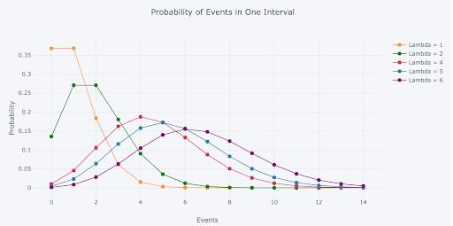
The most likely number of events in one interval for each curve is the curve’s rate parameter. This makes sense because the rate parameter is the expected number of events in one interval. Therefore, the rate parameter represents the number of events with the greatest probability when the rate parameter is an integer. When the rate parameter is not an integer, the highest probability number of events will be the nearest integer to the rate parameter. (The rate parameter is also the mean and variance of the distribution, which don’t need to be integers.)
Poisson Distribution Use Cases
Predicting Website Visits
Using the Poisson distribution, we could model the probability of seeing a certain amount of website visits in one day. For example, let’s say in one day, a given website is visited 10 times. From here, the Poisson distribution formula could determine how probable it is for the website to receive one visit, or possibly 100 visits, within another day’s period.
Predicting Hotel Bookings
The Poisson distribution can also be used to measure the probability of having a specific number of hotel bookings in one week. By observing 100 guests book rooms at a given hotel during a period of one week, this can then help predict the probability of getting 50, 75 or another amount of bookings at that same hotel in a week.
Predicting the Sales of a Product
Poisson distribution can also help provide the probability of how many of a certain product will be sold within one month. Let’s use a new smartphone model as an example. This smartphone model was sold 10,000 times in one month — so how probable is it that the model will sell 5,000 times in one month? Or maybe 20,000 times? The Poisson distribution formula could be applied here.
Poisson Distribution Example: Meteor Showers
We could continue with website failures to illustrate a problem solvable with a Poisson distribution, but I propose something grander. When I was a child, my father would sometimes take me into our yard to observe (or try to observe) meteor showers. We weren’t space geeks, but watching objects from outer space burn up in the sky was enough to get us outside, even though meteor showers always seemed to occur in the coldest months.
We can model the number of meteors seen as a Poisson distribution because the meteors are independent, the average number of meteors per hour is constant (in the short term), and — this is an approximation — meteors don’t occur at the same time.
All we need to characterize the Poisson distribution is the rate parameter, the number of events per interval * interval length. In a typical meteor shower, we can expect five meteors per hour on average or one every 12 minutes. Due to the limited patience of a young child (especially on a freezing night), we never stayed out more than 60 minutes, so we’ll use that as the time period. From these values, we get:

Five meteors expected mean that is the most likely number of meteors we’d observe in an hour. According to my pessimistic dad, that meant we’d see three meteors in an hour, tops. To test his prediction against the model, we can use the Poisson pmf distribution to find the probability of seeing exactly three meteors in one hour:

We get 14 percent or about 1/7. If we went outside and observed for one hour every night for a week, then we could expect my dad to be right once! We can use other values in the equation to get the probability of different numbers of events and construct the pmf distribution. Doing this by hand is tedious, so we’ll use Python calculation and visualization (which you can see in this Jupyter Notebook).
The graph below shows the probability mass function for the number of meteors in an hour with an average of 12 minutes between meteors, the rate parameter (which is the same as saying five meteors expected in an hour).
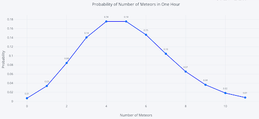
The most likely number of meteors is five, the rate parameter of the distribution. (Due to a quirk of the numbers, four and five have the same probability, 18 percent). There is one most likely value as with any distribution, but there is also a wide range of possible values. For example, we could see zero meteors or see more than 10 in one hour. To find the probabilities of these events, we use the same equation but, this time, calculate sums of probabilities (see notebook for details).
We already calculated the chance of seeing precisely three meteors as about 14 percent. The chance of seeing three or fewer meteors in one hour is 27 percent which means the probability of seeing more than 3 is 73 percent. Likewise, the probability of more than five meteors is 38.4 percent, while we could expect to see five or fewer meteors in 61.6 percent of hours. Although it’s small, there is a 1.4 percent chance of observing more than ten meteors in an hour!
To visualize these possible scenarios, we can run an experiment by having our sister record the number of meteors she sees every hour for 10,000 hours. The results are in the histogram below:
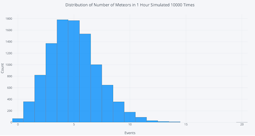
(This is just a simulation. No sisters were harmed in the making of this article.)
On a few lucky nights, we’d see 10 or more meteors in an hour, although more often, we’d see four or five meteors.
Experimenting With the Poisson Distribution Rate Parameter
The rate parameter, λ, is the only number we need to define the Poisson distribution. However, since it’s a product of two parts (events/interval * interval length), there are two ways to change it: we can increase or decrease the events/interval, and we can increase or decrease the interval length.
First, let’s change the rate parameter by increasing or decreasing the number of meteors per hour to see how those shifts affect the distribution. For this graph, we’re keeping the time period constant at 60 minutes.
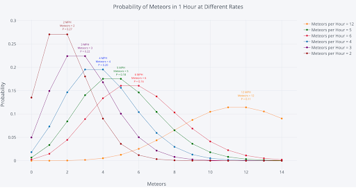
In each case, the most likely number of meteors in one hour is the expected number of meteors, the rate parameter. For example, at 12 meteors per hour (MPH), our rate parameter is 12, and there’s an 11 percent chance of observing exactly 12 meteors in one hour. If our rate parameter increases, we should expect to see more meteors per hour.
Another option is to increase or decrease the interval length. Here’s the same plot, but this time we’re keeping the number of meteors per hour constant at five and changing the length of time we observe.
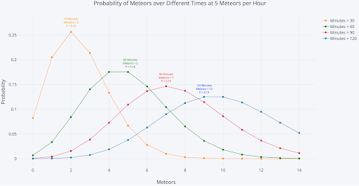
It’s no surprise that we expect to see more meteors the longer we stay out.
Using Poisson Distribution to Determine Poisson Process Waiting Time
An intriguing part of a Poisson process involves figuring out how long we have to wait until the next event (sometimes called the interarrival time). Consider the situation: meteors appear once every 12 minutes on average. How long can we expect to wait to see the next meteor if we arrive at a random time? My dad always (this time optimistically) claimed we only had to wait six minutes for the first meteor, which agrees with our intuition. Let’s use statistics and parts of the Poisson distribution formula to see if our intuition is correct.
I won’t go into the derivation (it comes from the probability mass function equation), but the time we can expect to wait between events is a decaying exponential. The probability of waiting a given amount of time between successive events decreases exponentially as time increases. The following equation shows the probability of waiting more than a specified time.

With our example, we have one event per 12 minutes, and if we plug in the numbers, we get a 60.65 percent chance of waiting more than six minutes. So much for my dad’s guess! We can expect to wait more than 30 minutes, about 8.2 percent of the time. (Note this is the time between each successive pair of events. The waiting times between events are memoryless, so the time between two events has no effect on the time between any other events. This memorylessness is also known as the Markov property).
A graph helps us to visualize the exponentially decaying probability of waiting time:
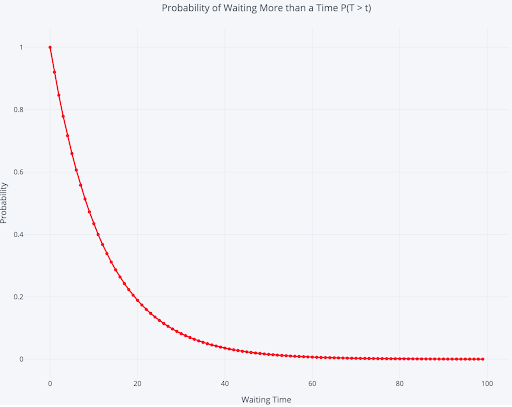
There is a 100 percent chance of waiting more than zero minutes, which drops off to a near-zero percent chance of waiting more than 80 minutes. Again, as this is a distribution, there’s a wide range of possible interarrival times.
Rearranging the equation, we can use it to find the probability of waiting less than or equal to a time:

We can expect to wait six minutes or less to see a meteor 39.4 percent of the time. We can also find the probability of waiting a length of time: There’s a 57.72 percent probability of waiting between 5 and 30 minutes to see the next meteor.
To visualize the distribution of waiting times, we can once again run a (simulated) experiment. We simulate watching for 100,000 minutes with an average rate of one meteor per 12 minutes. Then we find the waiting time between each meteor we see and plot the distribution.
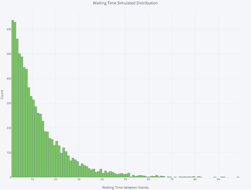
The most likely waiting time is one minute, but that’s distinct from the average waiting time. Let’s try to answer the question: On average, how long can we expect to wait between meteor observations?
To answer the average waiting time question, we’ll run 10,000 separate trials, each time watching the sky for 100,000 minutes, and record the time between each meteor. The graph below shows the distribution of the average waiting time between meteors from these trials:
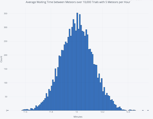
The average of the 10,000 runs is 12.003 minutes. Surprisingly, this average is also the average waiting time to see the first meteor if we arrive at a random time. At first, this may seem counterintuitive: if events occur on average every 12 minutes, then why do we have to wait the entire 12 minutes before seeing one event? The answer is we are calculating an average waiting time, taking into account all possible situations.
If the meteors came precisely every 12 minutes with no randomness in arrivals, then the average time we’d have to wait to see the first one would be six minutes. However, because waiting time is an exponential distribution, sometimes we show up and have to wait an hour, which outweighs the more frequent times when we wait fewer than 12 minutes. The average time to see the first meteor averaged over all the occurrences will be the same as the average time between events. The average first event waiting time in a Poisson process is known as the Waiting Time Paradox.
As a final visualization, let’s do a random simulation of one hour of observation.
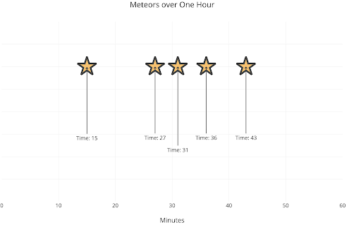
Well, this time we got precisely the result we expected: five meteors. We had to wait 15 minutes for the first one then 12 minutes for the next. In this case, it’d be worth going out of the house for celestial observation!
The next time you find yourself losing focus in statistics, you have my permission to stop paying attention to the teacher. Instead, find an interesting problem and solve it using the statistics you’re trying to learn. Applying technical concepts helps you learn the material and better appreciate how stats help us understand the world. Above all, stay curious: There are many amazing phenomena in the world, and data science is an excellent tool for exploring them.
Frequently Asked Questions
How do you know when to use a Poisson distribution?
You can use a Poisson distribution when you need to find the probability of a number of events happening within a given interval of time or space. These events must be occurring at random, independently of each other and at a constant average rate to be applicable for a Poisson distribution.
What is the criteria for a Poisson process?
For a process of events to be a Poisson process, these events must occur at a constant average rate, independently of each other and with no two events occurring at the same time.


