Mahalanobis Distance and Multivariate Outlier Detection in R

Mahalanobis distance is a metric that measures how far a point is from the center of a multivariate distribution, accounting for the covariance between variables. This makes it effective for detecting multivariate outliers and analyzing multivariate data.

In other words, Mahalanobis calculates the distance between point P1 and point P2 by considering how many standard deviations P1 is from P2. It also gives reliable results when outliers are considered as multivariate. 

In order to find outliers using the Mahalanobis distance, the distance between every point and center in n-dimension data are calculated and outliers found by considering these distances.

Mahalanobis vs. Euclidean Distance

Euclidean distance is also commonly used to find distance between two points in a two-, or more than two-dimensional space. But unlike Euclidean, Mahalanobis uses a covariance matrix. Because of that, Mahalanobis distance works well when two or more variables are highly correlated, even if their scales are not the same. When two or more variables are not on the same scale, Euclidean distance results might misdirect. When variables are on different scales, standardizing them (e.g., using Z-scores) improves the effectiveness of Euclidean distance. Moreover, Euclidean won’t work as well if the variables are highly correlated.

Let’s check out Euclidean and Mahalanobis formulas:

Mahalanobis distance incorporates the inverse of the covariance matrix to account for correlations among variables. As you can see from the formulas, Mahalanobis distance uses a covariance matrix (which is at the middle C ^(-1), unlike Euclidean). In the Euclidean formula, “p” and “q” represent the points whose distance will be calculated. The variable “n” represents the number of variables in multivariate data.

More on Data Science: The Fascinating World of Voronoi Diagrams

How to Find the Mahalanobis Distance Between Two Points

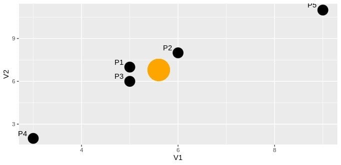
Suppose that we have five rows and two columns of data. As you can guess, every row in this data represents a point in a two-dimensional space.

      V1    V2
    ----- -----
 P1   5     7  
 P2   6     8  
 P3   5     6
 P4   3     2
 P5   9     11

Let’s draw a scatter plot of columns V1 and V2:

The orange point shows the center of these two variables (by mean), and the black points represent each row in the data frame. Now, let’s try to find Mahalanobis distance between P2 and P5:

According to the calculations above, the Mahalanobis distance between P2 and P5 is 4.08.

More on Data Science: The Ultimate Guide to Relational Operators in R

How to Find Outliers With Mahalanobis Distance in R

Mahalanobis distance is quite effective at finding outliers for multivariate data. If there are linear relationships between variables, Mahalanobis distance can figure out which observations break down the linearity. Unlike the other example, in order to find the outliers we need to find distance between each point and the center. The center point can be represented as the mean value of every variable in multivariate data.

In this example, we can use predefined data in R, which is called “airquality.” Using “Temp” and “Ozone” values as our variables, here is the list of steps that we need to follow:

• Find the center point of “Ozone” and “Temp.”
• Calculate the covariance matrix of “Ozone” and “Temp.”
• Find the Mahalanobis distance of each point to the center.
• Find the cut-off value from chi-square distribution.
• Select the distances that are less than cut-off. These are the values that aren’t outliers.

Below is the code to calculate the center and covariance matrix:

# Select only Ozone and Temp variables
air         = airquality[c("Ozone" , "Temp")]

# We need to remove NA from data set
air         = na.omit(air)

# Finding the center point 
air.center  = colMeans(air)

# Finding the covariance matrix
air.cov     = cov(air)

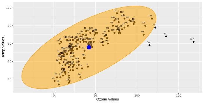
Before calculating the distances let’s plot our data and draw an ellipse by considering the center point and covariance matrix. We can find the ellipse coordinates by using the ellipse function that comes in the “car” package. 

The ellipse function takes three important arguments: center, shape and radius. Center represents the mean values of variables, shape represents the covariance matrix and radius should be the square root of chi-square value with two degrees of freedom and 0.95 probability. We take probability values 0.95 because anything outside the 0.95 will be considered an outlier, and the degree of freedom is two because we have two variables “Ozone” and “Temp.”

After our ellipse coordinates are found, we can create our scatter plot with “ggplot2” package:

# Call the package
library(ggplot2)

# Ellipse coordinates names should be same with air data set
ellipse <- as.data.frame(ellipse)
colnames(ellipse) <- colnames(air)

# Create scatter Plot
figure <- ggplot(air , aes(x = Ozone , y = Temp)) +
       geom_point(size = 2) +
       geom_polygon(data = ellipse , fill = "orange" , color = "orange" , alpha = 0.5)+
       geom_point(aes(air.center[1] , air.center[2]) , size = 5 , color = "blue") +
       geom_text( aes(label = row.names(air)) , hjust = 1 , vjust = -1.5 ,size = 2.5 ) +
       ylab("Temp Values") + xlab("Ozone Values")
       
# Run and display plot
figure

The above code snippet will return the scatter plot below:

The blue point on the plot shows the center point. Black points are the observations for Ozone and wind variables. As you can see, the points 30, 62, 117, 99 are outside the orange ellipse. It means that these points might be the outliers. If we consider that this ellipse has been drawn over covariance, center and radius, we can say we might have found the same points as the outlier for Mahalanobis distance. In Mahalanobis distance, we don’t draw an ellipse, but we calculate the distance between each point and center. After we find the distances, we use chi-square value as cut-off in order to identify outliers. This is the same as the radius of the ellipse in the above example.

The mahalanobis function that comes with R in the stats package returns distances between each point and the given center point. This function also takes three arguments: “x,” “center” and “cov.” As you can guess, “x” is multivariate data (matrix or data frame), “center” is the vector of center points of variables and “cov” is the covariance matrix of the data. This time, while obtaining the chi-square cut-off value, we shouldn’t take the square root. This is because Mahalanobis distance already returns D² (squared) distances, as you can see from the Mahalanobis distance formula.

# Finding distances
distances <- mahalanobis(x = air , center = air.center , cov = air.cov)

# Cutoff value for ditances from Chi-Sqaure Dist. 
# with p = 0.95 df = 2 which in ncol(air)
cutoff <- qchisq(p = 0.95 , df = ncol(air))

## Display observation whose distance greater than cutoff value
air[distances > cutoff ,]
## Returns : 30. 62. 99. 117. observations

Finally, we have identified the outliers in our multivariate data. The outliers are 30, 62, 99, 117 observations (rows), which are the same as the points outside of the ellipse in the scatter plot.

In this post, we’ve covered Mahalanobis distance from theory to practice. In addition to calculating the distance between two points using the formula, we also learned how to use it in order to find outliers in R. Although Mahalanobis distance isn’t used much in machine learning, it is very useful in defining multivariate outliers.

Frequently Asked Questions