If you have a background in electrical engineering, you’ve likely heard about Fourier transform. In basic terms, Fourier transform is a mathematical operation that changes the domain (x-axis) of a signal from time to frequency. The latter is particularly useful for decomposing a signal consisting of multiple pure frequencies.
What Is Fast Fourier Transform?
Fast fourier transform is an algorithm that determines the discrete Fourier transform of an object faster than computing it. This can be used to speed up training a convolutional neural network.
The application of Fourier transform isn’t limited to digital signal processing. Fourier transform can, in fact, speed up the training process of convolutional neural networks.
How Does Fast Fourier Transform Work?
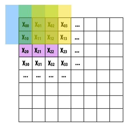
Recall how a convolutional layer overlays a kernel on a section of an image and performs bitwise multiplication with all of the values at that location. The kernel is then shifted to another section of the image and the process is repeated until it has traversed the entire image.
Fourier transform can speed up convolutions by taking advantage of the following property.

The above equation states that the convolution of two signals is equivalent to the multiplication of their Fourier transforms. Therefore, by transforming the input into frequency space, a convolution becomes a single element-wise multiplication. In other words, the input to a convolutional layer and kernel can be converted into frequencies using Fourier transform, multiplied once and then converted back using the inverse Fourier transform.
There is an overhead associated with transforming the inputs into the Fourier domain and the inverse Fourier transform to get responses back to the spatial domain. However, this is offset by the speed up obtained from performing a single multiplication instead of having to multiply the kernel with different sections of the image.
What Is Discrete Fourier Transform?
Discrete Fourier transform (DFT) can be written as follows.

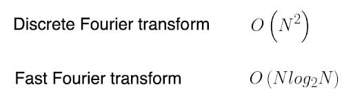
To determine the DFT of a discrete signal x[n] (where N is the size of its domain), we multiply each of its values by e raised to some function of n. We then sum the results obtained for a given n. If we used a computer to calculate the discrete Fourier transform of a signal, it would need to perform N (multiplications) x N (additions) = O(N²) operations.
As the name implies, fast Fourier transform (FFT) is an algorithm that determines the discrete Fourier transform of an input significantly faster than computing it directly. In computer science lingo, the FFT reduces the number of computations needed for a problem of size N from O(N^2) to O(NlogN).
On the surface, this might not seem like a big deal. However, when N is large enough, it can make a world of difference. Have a look at the following table.
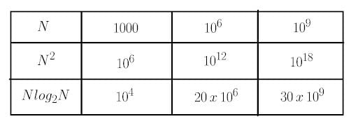
Say it took 1 nanosecond to perform one operation. It would take the fast Fourier transform algorithm approximately 30 seconds to compute the discrete Fourier transform for a problem of size N = 10⁹. In contrast, the regular algorithm would need several decades.

Fast Fourier Transform Algorithm
Suppose, we separated the Fourier transform into even and odd indexed sub-sequences.
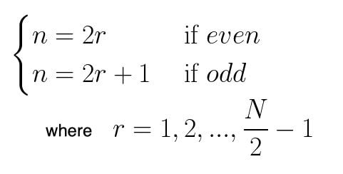
After performing a bit of algebra, we end up with the summation of two terms. The advantage of this approach lies in the fact that the even and odd indexed sub-sequences can be computed concurrently.
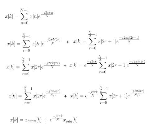
Suppose, N = 8 . To visualize the flow of data with time, we can make use of a butterfly diagram. We compute the discrete Fourier transform for the even and odd terms simultaneously. Then, we calculate x[k] using the formula from above.

We can express the gains in terms of Big O notation as follows. The first term comes from the fact that we compute the discrete Fourier transform twice. We multiply the latter by the time taken to compute the discrete Fourier transform on half the original input. In the final step, it takes N steps to add up the Fourier transform for a particular k. We account for this by adding N to the final product.

Notice how we were able to cut the time taken to compute the Fourier transform by a factor of two. We can further improve the algorithm by applying the divide-and-conquer approach, halving the computational cost each time. In other words, we can continue to split the problem size until we’re left with groups of two and then directly compute the discrete Fourier transforms for each of those pairs.

As long as N is a power of two, the maximum number of times you can split into two equal halves is given by p = log(N).

Here’s what it would look like if we were to use the fast Fourier transform algorithm with a problem size of N = 8. Notice how we have p = log(8) = 3 stages.

How to Implement Fast Fourier Transform in Python
Let’s take a look at how we could go about implementing the fast Fourier transform algorithm from scratch using Python. To begin, we import the numpy library.
import numpy as npNext, we define a function to calculate the discrete Fourier transform directly.
def dft(x):
    x = np.asarray(x, dtype=float)
    N = x.shape[0]
    n = np.arange(N)
    k = n.reshape((N, 1))
    M = np.exp(-2j * np.pi * k * n / N)
    return np.dot(M, x)
We can ensure our implementation is correct by comparing the results with those obtained from NumPy’s fft function.
x = np.random.random(1024)
np.allclose(dft(x), np.fft.fft(x))

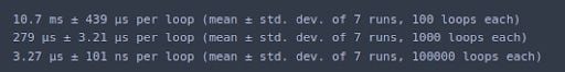
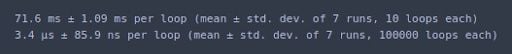
As we can clearly see, the discrete Fourier transform function is orders of magnitude slower than the fast Fourier transform algorithm.
%timeit dft(x)
%timeit np.fft.fft(x)

As we saw before, the fast Fourier transform works by computing the discrete Fourier transform for small subsets of the overall problem and then combining the results. The latter can easily be done in code using recursion.
def fft(x):
    x = np.asarray(x, dtype=float)
    N = x.shape[0]
    if N % 2 > 0:
        raise ValueError("must be a power of 2")
    elif N <= 2:
        return dft(x)
    else:
        X_even = fft(x[::2])
        X_odd = fft(x[1::2])
        terms = np.exp(-2j * np.pi * np.arange(N) / N)
        return np.concatenate([X_even + terms[:int(N/2)] * X_odd,
                               X_even + terms[int(N/2):] * X_odd])
Again, we can validate whether our implementation is correct by comparing the results with those obtained from NumPy.
x = np.random.random(1024)
np.allclose(fft(x), np.fft.fft(x))

The FFT algorithm is significantly faster than the direct implementation. However, it still lags behind the NumPy implementation by quite a bit. One reason for this is the fact that the NumPy implementation uses matrix operations to calculate the Fourier transforms simultaneously.
%timeit dft(x)
%timeit fft(x)
%timeit np.fft.fft(x)
We define another function to compute the Fourier transform. Only this time around, we make use of vector operations instead of recursion.
def fft_v(x):
    x = np.asarray(x, dtype=float)
    N = x.shape[0]
    if np.log2(N) % 1 > 0:
        raise ValueError("must be a power of 2")

    N_min = min(N, 2)

    n = np.arange(N_min)
    k = n[:, None]
    M = np.exp(-2j * np.pi * n * k / N_min)
    X = np.dot(M, x.reshape((N_min, -1)))
while X.shape[0] < N:
        X_even = X[:, :int(X.shape[1] / 2)]
        X_odd = X[:, int(X.shape[1] / 2):]
        terms = np.exp(-1j * np.pi * np.arange(X.shape[0])
                        / X.shape[0])[:, None]
        X = np.vstack([X_even + terms * X_odd,
                       X_even - terms * X_odd])
return X.ravel()
Once again, we can ensure we obtained the correct results by comparing them with those from the NumPy library.
x = np.random.random(1024)
np.allclose(fft_v(x), np.fft.fft(x))

As we can see, the FFT implementation using vector operations is significantly faster than what we had obtained previously. We still haven’t come close to the speed at which the NumPy library computes the Fourier transform. This is because the FFTPACK algorithm behind NumPy’s fft is a Fortran implementation, which has received years of tweaks and optimizations. If you are interested in finding out more, I recommend you have a look at the source code.
%timeit fft(x)
%timeit fft_v(x)
%timeit np.fft.fft(x)