Big O notation is a metric used in computer science to classify algorithms based on their time and space complexity. The time and space here is not based on the actual number of operations performed or the amount of memory used per se, but rather how the algorithm would scale with an increase or decrease in the amount of input data.
What Is Big O Notation?
Big O notation generally represents how an algorithm will run in a worst-case scenario, in other words what the maximum time or space an algorithm could use is. The complexity can be written as O(x), where x is the growth rate of the algorithm in regards to n, which is the amount of data input. Throughout the rest of this post, input will be referred to as n.
Types of Big O Notations
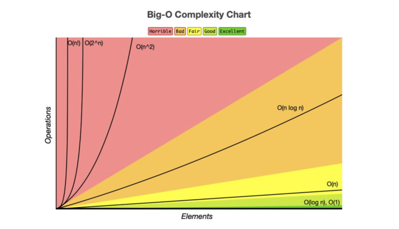
There are seven common types of big O notations. These include:
- O(1): Constant complexity.
- O(logn): Logarithmic complexity.
- O(n): Linear complexity.
- O(nlogn): Loglinear complexity.
- O(n^x): Polynomial complexity.
- O(X^n): Exponential time.
- O(n!): Factorial complexity.
Let’s examine each one.
O(1): Constant Complexity
O(1) is known as constant complexity. This implies that the algorithm’s time or space complexity remains constant regardless of the input size n, and the amount of time or memory does not scale with n. For time complexity, this means that n is not iterated on or recursed. Generally, a value will be selected and returned, or a value will be operated on and returned.

For space, no data structures can be created that are multiples of the size of n, as space usage does not increase with the size of the input. Variables can be declared, but the number must not change with n.

O(logn): Logarithmic Complexity
O(logn) is known as logarithmic complexity. The logarithm in O(logn) typically has a base of two. The best way to wrap your head around this is to remember the concept of halving. Every time n increases by an amount k, the time or space increases by k/2. There are several common algorithms that are O(logn) a vast majority of the time, including: binary search, searching for a term in a binary search tree and adding items to a heap.

O(logn) space complexity commonly happens during recursive algorithms where the recursion depth is logarithmic (like in binary search). When a recursive call is made, all current variables get placed on the stack and new ones are created. If the number of recursive calls increases logarithmically, i.e., n is halved with every recursive call, then the space complexity will be O(logn). Space complexities of O(logn) are rarer to encounter.

O(n): Linear Complexity
O(n), or linear complexity, is perhaps the most straightforward complexity to understand. O(n) means that the time/space scales 1:1 with changes to the size of n. If a new operation or iteration is needed every time n increases by one, then the algorithm will run in O(n) time.

When using data structures, if one more element is needed every time n increases by one, then the algorithm will use O(n) space.

O(nlogn): Loglinear Complexity
O(nlogn) is known as loglinear complexity. O(nlogn) implies that logn operations will occur n times. In other words, for each of the n elements, a logarithmic operation is done. O(nlogn) time is common in recursive sorting algorithms, binary tree sorting algorithms and most other types of sorts.
Nlogn Defined

Space complexities of O(nlogn) are extremely rare to the point that you don’t need to keep an eye out for it. Any algorithm that uses O(nlogn) space will likely be awkward enough that it will be apparent.

O(nˣ): Polynomial Complexity
O(nˣ), or polynomial complexity, covers a larger range of complexities depending on the value of x. X represents the number of times all of n will be processed for every n. Polynomial complexity is where we enter the danger zone. It’s extremely inefficient, and while it is the only way to create some algorithms, polynomial complexity should be regarded as a “warning sign” that the code can be refactored. This holds true for not just polynomial complexity, but for all following complexities we will cover.
A red flag that an algorithm will run in polynomial time is the presence of nested loops. A general rule of thumb is that x will equal the number of nested loops. A major exception to this rule is when you are working with matrices and multi-dimensional arrays. Nested loops are needed to traverse these data structures and do not represent polynomial time. Polynomial time will require the number of loops to equal 2y, where y is the number of dimensions present in the data structure.

For nested loops to create polynomial time complexity, all loops must be iterating over n.

Polynomial space complexity will generally be because of the creation of a matrix or multidimensional array in a function creating a table.

O(Xⁿ): Exponential Time
O(Xⁿ), known as exponential time, means that time or space will be raised to the power of n. Exponential time is extremely inefficient and should be avoided unless absolutely necessary. Often O(Xⁿ) results from having a recursive algorithm that calls X number of algorithms with n-1. Towers of Hanoi is a famous problem that has a recursive solution running in O(2ⁿ).

You will likely never encounter algorithms using a space complexity of O(Xⁿ) in standard software engineering. It can be encountered when using Turing machines and the arithmetic model of computation, but this is extremely hard to implement using a JavaScript example, and beyond the scope of this article. Suffice to say, if O(Xⁿ) space complexity is ever encountered, it’s likely that something has gone horribly, horribly wrong.
O(n!): Factorial Complexity
O(n!), or factorial complexity, is the “worst” standard complexity that exists. To illustrate how fast factorial solutions will blow up in size, a standard deck of cards has 52 cards, with 52! possible orderings of cards after shuffling. This number is larger than the number of atoms on Earth. If someone were to shuffle a deck of cards every second from the beginning of the universe until the present second, they would not have encountered every possible ordering of a deck of cards. It is highly unlikely that any current deck of shuffled cards you encounter has ever existed in that order in history. To sum up: Factorial complexity is unimaginably inefficient.
An algorithm with exponential time complexity is the brute force solution to the traveling salesman problem. Although, a more efficient algorithm has been discovered to solve this in exponential time using the Held-Karp algorithm. If you can figure out an efficient solution, you will be a rich person, netting a $2,000,000 prize.

The only algorithms I can find that have O(n!) space complexity involve the security of RFID tags in robotics. The algorithms are made purposefully complex to thwart efforts to compute a solution. I do not understand exactly how these work, which probably bodes well for the security they are trying to implement.
Why Big O Notations Are Important to Know
The first four complexities discussed here, and to some extent the fifth, O(1), O(logn), O(n), O(nlogn) and O(nˣ), can be used to describe the vast majority of algorithms you’ll encounter. The final two will be exceedingly rare but are important to understand to grasp the whole of Big O notation and what it’s used to represent. There are also other, minor complexities that exists out there, such as double logarithmic (O(loglogn)) and fractional power (O(nˣ) 0 < x < 1), among others, however these are a bit niche and will not be applicable to a large portion of algorithms.
Frequently Asked Questions
What is Big O notation?
Big O notation is a mathematical concept used to describe the time and space complexity of algorithms, showing how an algorithm's performance scales with the size of the input data. Big O notation can help gauge how different algorithms will perform as data grows, and how to optimize software in specific scenarios.
What is the difference between O(1) and O(n) complexity?
O(1) refers to constant complexity, where the algorithm’s performance is not affected by the input size, while O(n) refers to linear complexity, where algorithm performance scales linearly with the input size.
What is the meaning of O(nlogn)?
O(nlogn) represents loglinear complexity, which occurs when an algorithm performs logarithmic operations for each of the n elements, commonly seen in sorting algorithms like quicksort.