DBSCAN Clustering Algorithm Demystified

Density-based spatial clustering of applications with noise (DBSCAN) is a popular clustering algorithm used in machine learning and data mining to group points in a data set that are closely packed together based on their distance to other points.

DBSCAN works by partitioning the data into dense regions of points that are separated by less dense areas. It defines clusters as areas of the data set where there are many points close to each other, while the points that are far from any cluster are considered outliers or noise.

How Does DBSCAN Work?

To understand how the algorithm works, we will walk through a simple example. Let’s say we have a data set of points like the following:

Our goal is to cluster these points into groups that are densely packed together. First, we count the number of points close to each point. For example, if we start with the green point, we draw a circle around it.

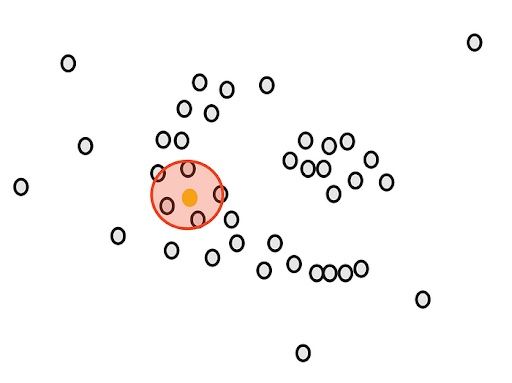
The radius ε (epsilon) of the circle is the first parameter that we have to determine when using DBSCAN.

After drawing the circle, we count the overlaps. For example, for our yellow point, there are five close points.

Likewise, we count the number of close points for all remaining points.

Next, we will determine another parameter, the minimum number of points m. Each point is considered a core point if they are close to at least m other points. For example, if we take m as three, then, purple points are considered as core points, but the yellow one is not because it doesn’t have any close points around it.

Then, we randomly select a core point and assign it as the first point in our first cluster. Other points that are close to this point are also assigned to the same cluster (i.e., within the circle of the selected point).

Then, we extend it to the other points that are close.

We stop when we can’t assign more core points to the first cluster. Some core points couldn’t be appointed even though they were close to the first cluster. We draw the circles of these points and see if the first cluster is close to the core points. If there is an overlap, we put them in the first cluster.

However, we can’t assign any non-core points. They are considered outliers.

Now, we still have core points that aren’t assigned. We randomly select another point from them and start over.

DBSCAN works sequentially, so it’s important to note that non-core points will be assigned to the first cluster that meets the requirement of closeness.

More on Machine LearningK-Nearest Neighbor Algorithm: An Introduction

How to Implement DBSCAN in Python 

We can use the DBSCAN class from Sklearn. Before implementing any model, Let’s get to know the DBSCAN class better. We can pass some arguments to the object.

• eps: The maximum distance between two points for them to be considered neighbors. Points that are within eps distance of each other are considered part of the same cluster.
• min_samples: The minimum number of points required for a point to be considered a core point. Points that have fewer than min_samples neighbors are labeled as noise.
• metric: The distance metric used to measure the distance between points. By default, Euclidean distance is used, but other metrics such as Manhattan distance or cosine distance can be used.
• algorithm: The algorithm used to compute the nearest neighbors of each point. The default is "auto", which selects the most appropriate algorithm based on the size and dimensionality of the data. Other options include "ball_tree", "kd_tree"and "brute".
• leaf_size: The size of the leaf nodes used in the ball_tree or kd_tree algorithms. Smaller leaf size results in a more accurate but slower tree construction.
• p: The power parameter for the Minkowski distance metric. When p=1, this is equivalent to the Manhattan distance, and when p=2, this is equivalent to the Euclidean distance.
• n_jobs: The number of CPU cores to use for parallel computation. Set to -1 to use all available cores.

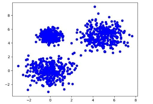
Now, let’s generate some dummy data.

import matplotlib.pyplot as plt
from sklearn.datasets import make_blobs

# generation of nested dummy data
X, y = make_blobs(n_samples=1000, centers=[[0, 0], [0, 5], [5, 5]], cluster_std=[1.0, 0.5, 1.0])

plt.scatter(X[:,0], X[:,1], color='blue')
plt.show()

And the model:

from sklearn.cluster import DBSCAN

# model
dbscan = DBSCAN(eps=0.5, min_samples=5)
labels = dbscan.fit_predict(X)

# the number of clusters found by DBSCAN
n_clusters = len(set(labels)) - (1 if -1 in labels else 0)
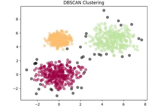
print(f"Number of clusters found by DBSCAN: {n_clusters}")
# Number of clusters found by DBSCAN: 3

Now, let’s plot the clsuters.

import numpy as np

unique_labels = set(labels)
colors = [plt.cm.Spectral(each) for each in np.linspace(0, 1, len(unique_labels))]
for k, col in zip(unique_labels, colors):
    if k == -1:
        col = [0, 0, 0, 1]  # Black color for noise points (label=-1)
    class_member_mask = (labels == k)
    xy = X[class_member_mask]
    plt.scatter(xy[:, 0], xy[:, 1], s=50, c=[col], marker='o', alpha=0.5)

plt.title('DBSCAN Clustering')
plt.show()

# attributes of the dbscan object
print("Indices of core samples: ", dbscan.core_sample_indices_)
print("Copy of each core sample found by training: ", dbscan.components_)
print("Labels: ", dbscan.labels_)
print("Number of features seen during fit: ", dbscan.n_features_in_)

DBSCAN Advantages

DBSCAN has several strengths that make it a popular clustering algorithm for many types of data sets and clustering tasks. It’s capable of identifying clusters of any shape, making it more versatile than k-means or hierarchical clustering.

It’s also robust to noise, meaning it can effectively identify and ignore noise points that don’t belong to any cluster. This makes it a useful tool for data cleaning and outlier detection.

It’s a parameter-free clustering algorithm, meaning that it doesn’t require the user to specify the number of clusters in advance. This can be a major advantage in scenarios where the optimal number of clusters is unknown or difficult to determine.

Finally, DBSCAN is efficient on large data sets with a time complexity of O(nlogn), making it a scalable algorithm for data with millions of points.

More on Machine LearningC-Means Clustering Algorithm Explained

DBSCAN Disadvantages

Despite its many strengths, DBSCAN also has several weaknesses. Its performance can be sensitive to the choice of hyperparameters, particularly eps and min_samples, which can require some trial and error to find optimal values.

DBSCAN may perform poorly on data sets with clusters of significantly different densities. This is because the optimal eps value for one cluster may be too large or too small for another cluster, leading to poor cluster identification.

DBSCAN’s performance can be limited on high-dimensional data due to the curse of dimensionality, where the distance between points becomes less meaningful in high-dimensional spaces. This can lead to poor cluster identification and may require dimensionality reduction techniques to be used in conjunction with DBSCAN.