Beginner’s Guide to VGG16 Implementation in Keras

VGG16 is a convolutional neural network (CNN) architecture that’s considered to be one of the best computer vision model architectures to date. It specializes in image classification and image recognition for a wide range of images.

What Is VGG16?

VGG16 is a deep convolutional neural network model used for image classification tasks. The network is composed of 16 layers of artificial neurons, which each work to process image information incrementally and improve the accuracy of its predictions.

Instead of having a large number of hyper-parameters, VGG16 uses convolution layers with a 3x3 filter and a stride 1 that are in the same padding and maxpool layer of 2x2 filter of stride 2. It follows this arrangement of convolution and max pool layers consistently throughout the whole architecture. In the end it has two fully connected layers, followed by a softmax for output. 

In VGG16, ‘VGG’ refers to the Visual Geometry Group of the University of Oxford, while the ‘16’ refers to the network’s 16 layers that have weights. This network is a pretty large network, and it has about 138 million parameters.

How Is VGG16 Used?

VGG16 is used for image recognition and classification in new images. The pre-trained version of the VGG16 network is trained on over one million images from the ImageNet visual database, and is able to classify images into 1,000 different categories with 92.7 percent top-5 test accuracy. VGG16 can be applied to determine whether an image contains certain items, animals, plants and more.

More on Machine Learning: How Does Backpropagation in a Neural Network Work? 

How to Implement VGG16 in Keras

We’re going to implement full VGG16 from scratch in Keras using the “Dogs vs. Cats” data set. Once you’ve downloaded the images, you can follow along with the steps written below.

1. Import the Libraries for VGG16

import keras,os
from keras.models import Sequential
from keras.layers import Dense, Conv2D, MaxPool2D , Flatten
from keras.preprocessing.image import ImageDataGenerator
import numpy as np

Let’s start with importing all the libraries that you will need to implement VGG16. In this example, we’ll be using the sequential method, as we’re creating a sequential model. A sequential model means that all the layers of the model will be arranged in sequence. 

We’ll import ImageDataGenerator from keras.preprocessing. The objective of ImageDataGenerator is to make it easier to import data with labels into the model. It’s a useful class, as it comes with a variety of functions that allow you to rescale, rotate, zoom and flip, etc. The most useful thing about this class is that it doesn’t affect the data stored on the disk. This class alters the data on the go while passing it to the model.

trdata = ImageDataGenerator()
traindata = trdata.flow_from_directory(directory="data",target_size=(224,224))
tsdata = ImageDataGenerator()
testdata = tsdata.flow_from_directory(directory="test", target_size=(224,224))

More on Machine Learning: Image Classification With MobileNet

2. Create an Object for Training and Testing Data

Next, we’ll create an object of ImageDataGenerator for both training and testing data and passing the folder, which has train data, to the object trdata, and similarly passing the folder, which has test data, to the object tsdata. The folder structure of the data will be as follows:

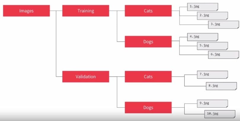
The ImageDataGenerator will automatically label all the data inside cat folder as cat and vis-à-vis for dog folder. In this way data is easily ready to be passed to the neural network.

model = Sequential()
model.add(Conv2D(input_shape=(224,224,3),filters=64,kernel_size=(3,3),padding="same", activation="relu"))
model.add(Conv2D(filters=64,kernel_size=(3,3),padding="same", activation="relu"))
model.add(MaxPool2D(pool_size=(2,2),strides=(2,2)))
model.add(Conv2D(filters=128, kernel_size=(3,3), padding="same", activation="relu"))
model.add(Conv2D(filters=128, kernel_size=(3,3), padding="same", activation="relu"))
model.add(MaxPool2D(pool_size=(2,2),strides=(2,2)))
model.add(Conv2D(filters=256, kernel_size=(3,3), padding="same", activation="relu"))
model.add(Conv2D(filters=256, kernel_size=(3,3), padding="same", activation="relu"))
model.add(Conv2D(filters=256, kernel_size=(3,3), padding="same", activation="relu"))
model.add(MaxPool2D(pool_size=(2,2),strides=(2,2)))
model.add(Conv2D(filters=512, kernel_size=(3,3), padding="same", activation="relu"))
model.add(Conv2D(filters=512, kernel_size=(3,3), padding="same", activation="relu"))
model.add(Conv2D(filters=512, kernel_size=(3,3), padding="same", activation="relu"))
model.add(MaxPool2D(pool_size=(2,2),strides=(2,2)))
model.add(Conv2D(filters=512, kernel_size=(3,3), padding="same", activation="relu"))
model.add(Conv2D(filters=512, kernel_size=(3,3), padding="same", activation="relu"))
model.add(Conv2D(filters=512, kernel_size=(3,3), padding="same", activation="relu"))
model.add(MaxPool2D(pool_size=(2,2),strides=(2,2)))

3. Initialize the Model

Next, we’ll start initializing the model by specifying that it’s a sequential model. After that, we’ll add:

• 2 x convolution layer of 64 channel of 3x3 kernel and same padding.
• 1 x maxpool layer of 2x2 pool size and stride 2x2.
• 2 x convolution layer of 128 channel of 3x3 kernel and same padding.
• 1 x maxpool layer of 2x2 pool size and stride 2x2.
• 3 x convolution layer of 256 channel of 3x3 kernel and same padding.
• 1 x maxpool layer of 2x2 pool size and stride 2x2.
• 3 x convolution layer of 512 channel of 3x3 kernel and same padding.
• 1 x maxpool layer of 2x2 pool size and stride 2x2.
• 3 x convolution layer of 512 channel of 3x3 kernel and same padding.
• 1 x maxpool layer of 2x2 pool size and stride 2x2.

We also added the rectified linear unit (ReLU) activation to each layer so that the negative values aren’t passed to the next layer.

model.add(Flatten())
model.add(Dense(units=4096,activation="relu"))
model.add(Dense(units=4096,activation="relu"))
model.add(Dense(units=2, activation="softmax"))

4. Pass the Data to the Dense Layer

After creating all the convolutions, we’ll pass the data to the dense layer. For that, we’ll flatten the vector that came out of the convolutions and add:

• 1 x Dense layer of 4096 units.
• 1 x Dense layer of 4096 units.
• 1 x Dense Softmax layer of two units.

We’ll use the ReLU activation for both the dense layer of 4096 units to prevent forwarding negative values through the network. We’ll use a two-unit dense layer in the end with Softmax activation, as we have two classes to predict from in the end, which are dog and cat. The Softmax layer will output the value between 0 and 1 based on the confidence of the model depending on the class the images belong to.

After creating the Softmax layer, the model is finally prepared. Now, we need to compile the model.

More on Machine Learning: 5 Neural Network Activation Functions to Know

5. Compile the Model

from keras.optimizers import Adam
opt = Adam(lr=0.001)
model.compile(optimizer=opt, loss=keras.losses.categorical_crossentropy, metrics=['accuracy'])

Here, we’ll be using the Adam optimizer to reach the global minima while training the model. The Adam optimizer will help us to get out of local minima and reach global minima if we get stuck while training. We’ll also specify the learning rate of the optimizer, in this case, it’s set at 0.001. If our training bounces a lot on epochs, then we need to decrease the learning rate so that we can reach global minima.

We can check the summary of the model that we created by using the code below.

model.summary()

The output of this will be the summary of the model we just created.

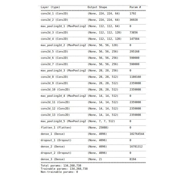
from keras.callbacks import ModelCheckpoint, EarlyStopping
checkpoint = ModelCheckpoint("vgg16_1.h5", monitor='val_acc', verbose=1, save_best_only=True, save_weights_only=False, mode='auto', period=1)
early = EarlyStopping(monitor='val_acc', min_delta=0, patience=20, verbose=1, mode='auto')
hist = model.fit_generator(steps_per_epoch=100,generator=traindata, validation_data= testdata, validation_steps=10,epochs=100,callbacks=[checkpoint,early])

6. Import Libraries to Monitor and Control Training

After the creation of the model, we’ll import ModelCheckpoint and the EarlyStopping method from Keras. We’ll create an object of both and pass that as callback functions to fit_generator.

ModelCheckpoint allows us to save the model by monitoring a specific parameter. In this case, we are monitoring validation accuracy by passing val_acc to ModelCheckpoint. The model will only be saved to the disk if the validation accuracy of the model in its current epoch is greater than what it was in the last epoch.

EarlyStopping helps us to stop the training of the model early if there is no increase in the parameter that we’ve set to monitor in EarlyStopping. In this case, we are monitoring validation accuracy by passing val_acc to EarlyStopping. We have here set patience to 20, which means that the model will stop training if it doesn’t see any rise in validation accuracy in 20 epochs.

We’ll use a model.fit_generator, as we are using ImageDataGenerator to pass data to the model. We will pass train and test data to fit_generator. fit_generator steps_per_epoch will set the batch size to pass training data to the model and validation_steps will do the same for test data. We can tweak it based on our system specifications.

After executing the above line, the model will start to train and we’ll start to see the training/validation accuracy and loss.

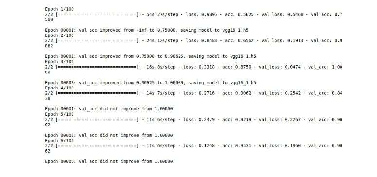
7. Visualize the Training/Validation Data

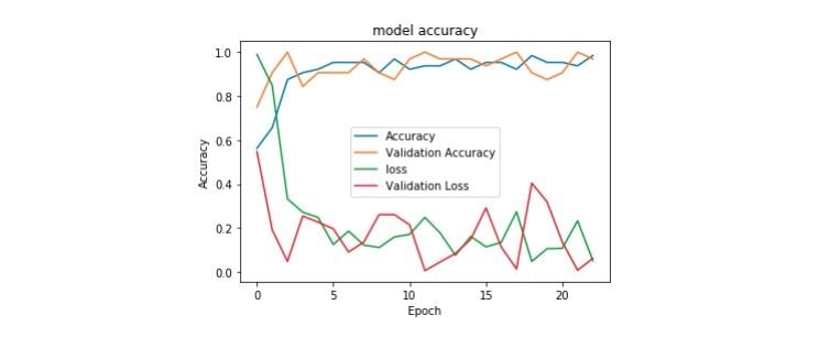
Once we’ve trained the model, we can visualize the training/validation accuracy and loss. As you may have noticed, we are passing the output of mode.fit_generator to the hist variable. All the training/validation accuracy and loss are stored in hist, and we’ll visualize it from there.

import matplotlib.pyplot as plt
plt.plot(hist.history["acc"])
plt.plot(hist.history['val_acc'])
plt.plot(hist.history['loss'])
plt.plot(hist.history['val_loss'])
plt.title("model accuracy")
plt.ylabel("Accuracy")
plt.xlabel("Epoch")
plt.legend(["Accuracy","Validation Accuracy","loss","Validation Loss"])
plt.show()

Here we’ll visualize training/validation accuracy and loss using Matplotlib.

8. Test Your Model

To do predictions on the trained model, we need to load the best saved model and pre-process the image and pass the image to the model for output.

from keras.preprocessing import image
img = image.load_img("image.jpeg",target_size=(224,224))
img = np.asarray(img)
plt.imshow(img)
img = np.expand_dims(img, axis=0)
from keras.models import load_model
saved_model = load_model("vgg16_1.h5")
output = saved_model.predict(img)
if output[0][0] > output[0][1]:
    print("cat")
else:
    print('dog')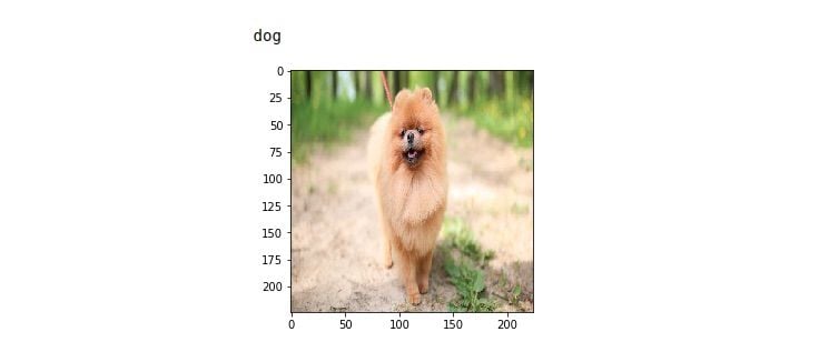

Here, we’ve loaded the image using the image method in Keras, converted it to a numpy array and added an extra dimension to the image for matching in NHWC (Number, Height, Width, Channel) format of k=Keras.

This is a complete implementation of VGG16 in Keras using ImageDataGenerator. We can make this model work for any number of classes by changing the unit of the last Softmax dense layer to whatever number we want based on the classes which we need to classify.

If you have less data, then instead of training your model from scratch, you can try transfer learning. 

Frequently Asked Questions