Image Classification With MobileNet

MobileNet is a light-weight computer vision model designed to be used in mobile applications. 

 This article covers five parts:

1. What is MobileNet?
2. MobileNet depthwise separable convolution explained.
3. Difference between MobileNet and traditional convolutional neural network (CNN) 
4. MobileNet with Python Example.
5. Advantages of MobileNet.

What Is MobileNet?

MobileNet is TensorFlow’s first mobile computer vision model. It is a class of convolutional neural network (CNN) that was open-sourced by Google, and therefore, provides an excellent starting point for training classifiers that are compact yet fast and efficient in performance.

The speed and power consumption of the MobileNet network is proportional to the number of multiply-accumulates (MACs) which is a measure of the number of fused multiplication and addition operations.

MobileNet uses depthwise separable convolutions to significantly reduce the number of parameters compared to other networks with regular convolutions and the same depth in the nets. This results in lightweight deep neural networks.

More on Machine Learning: NLP for Beginners: A Complete Guide

MobileNet Depthwise Separable Convolution Explained

Depthwise separable convolution originated from the idea that a filter’s depth and spatial dimension can be separated, thus, the name separable.

A depthwise separable convolution is made from two operations:

1. Depthwise convolution.
2. Pointwise convolution.

Let’s take the example of the Sobel filter used in image processing to detect edges.

You can separate the height and width dimensions of these filters. Gx filter can be viewed as a matrix product of [1 2 1] transpose with [-1 0 1].

You’ll notice that the filter has disguised itself. It shows it had nine parameters, but it has six. This is possible because of the separation of its height and width dimensions.

The same idea applies to a separate depth dimension from horizontal (width*height), which gives us a depthwise separable convolution where we perform depthwise convolution. After that, we use a 1*1 filter to cover the depth dimension.

One thing to notice is how much the parameters are reduced by this convolution to output the same number of channels. To produce one channel, we’d need 3*3*3 parameters to perform depth-wise convolution and 1*3 parameters to perform further convolution in-depth dimension.

But if we’d need three output channels, we’d only need three 1*3 depth filters, giving us a total of 36 (= 27 + 9) parameters. Meanwhile, for the same number of output channels in regular convolution, we’d need three 3*3*3 filters, giving us a total of 81 parameters.

In the context of depthwise convolution:

• DK is the spatial dimension of the kernel
• DF is the spatial width and height of the input feature map
• M is the number of input channels 
• N is the number of output channels

Depthwise separable convolution is a depthwise convolution followed by a pointwise convolution, as follows:

1. Depthwise convolution is the channel-wise DK×DK spatial convolution, where DK×DK represents the size of the convolution in each channel of the input image. Suppose we have five channels, we’d then have five DK×DK spatial convolutions.
2. Pointwise convolution is the 1×1 convolution to change the dimension.

Depthwise is a map of a single convolution on each input channel separately. Therefore, its number of output channels is the same as the number of the input channels. Its computational cost is: DF² * M * DK².

Pointwise Convolution

Pointwise convolution is a convolution with a kernel size of 1x1 that simply combines the features created by the depthwise convolution. Its computational cost is: M * N * DF².

Difference Between MobileNet and Traditional Convolutional Neural Network (CNN) 

The main difference between a traditional CNN and the MobileNet architecture is that a traditional CNN applies a standard convolution to each input and output channel, while MobileNet uses a depthwise separable convolution operation, which splits the operation into a depthwise convolution and a pointwise convolution. For example, instead of using a single 3x3 convolution layer, MobileNet splits the convolution operation into a 3x3 depthwise convolution and a 1x1 pointwise convolution.

MobileNet With Python Example

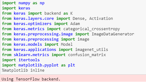
Below is an example of MobileNet with Python. 

mobile = keras.applications.mobilenet.MobileNet()

def prepare_image(file):
    img = image.load_img(file, target_size=(224, 224))
    img_array = image.img_to_array(img)
    img_array_expanded_dims = np.expand_dims(img_array, axis=0)
    return keras.applications.mobilenet.preprocess_input(img_array_expanded_dims)

from IPython.display import Image
Image(filename='click.jpg', width=250,height=300)

preprocessed_image = prepare_image('click.jpg') 
predictions = mobile.predict(preprocessed_image) 
results = imagenet_utils.decode_predictions(predictions)

print(results)

This creates the output:

More on Machine Learning: Understanding Cosine Similarity and Its Applications

Advantages of MobileNet

MobileNets are a family of mobile-first computer vision models for TensorFlow, designed to effectively maximize accuracy while being mindful of the restricted resources for an on-device or embedded application.

MobileNets are small, low-latency, low-power models parameterized to meet the resource constraints of a variety of use-cases. They can be built upon for classification, detection, embeddings and segmentation tasks.

Frequently Asked Questions