How to Practice Word2Vec for NLP Using Python

When brainstorming new data science topics to investigate, I always gravitate towards Natural Language Processing (NLP). It is a rapidly growing field of data science with constant innovations to explore; plus, I love to analyze writing and rhetoric. NLP naturally fits my interests! Previously, I wrote an article about simple projects to get started in NLP using the bag of words models. This article goes beyond the simple bag of words approaches by exploring quick and easy ways to generate word embeddings using word2vec through the Python Gensim library.

Bag of Words vs. Word2Vec

When I started exploring NLP, the first models I learned about were simple bag of words models. Although they can be very effective, they have limitations.

The Traditional Bag of Words Approach

A bag of words (BoW) is a representation of text that describes the occurrence of words within a text corpus, but doesn’t account for the sequence of the words. That means it treats all words independently from one another, hence the name bag of words.

BoW consists of a set of words (vocabulary) and a metric like frequency or term frequency-inverse document frequency (TF-IDF) to describe each word’s value in the corpus. That means BoW can result in sparse matrices and high dimensional vectors that consume a lot of computer resources if the vocabulary is very large.

To simplify the concept of BoW vectorization, imagine you have two sentences:

• The dog is white
• The cat is black

Converting the sentences to a vector space model would transform them in such a way that looks at the words in all sentences, and then represents the words in the sentence with a number. If the sentences were one-hot encoded:

• The dog cat is white black
• The dog is white = [1,1,0,1,1,0]
• The cat is black = [1,0,1,1,0,1]

The BoW approach effectively transforms the text into a fixed-length vector to be used in machine learning.

Want to Practice BoW? We Got You.3 Ways to Learn Natural Language Processing Using Python

The Word2Vec Approach

Developed by a team of researchers at Google, word2vec attempts to solve a couple of the issues with the BoW approach:

• High-dimension vectors
• Words assumed completely independent of each other

Using a neural network with only a couple layers, word2vec tries to learn relationships between words and embeds them in a lower-dimensional vector space. To do this, word2vec trains words against other words that neighbor them in the input corpus, capturing some of the meaning in the sequence of words. The researchers devised two novel approaches:

• Continuous bag of words (CBoW)
• Skip-gram

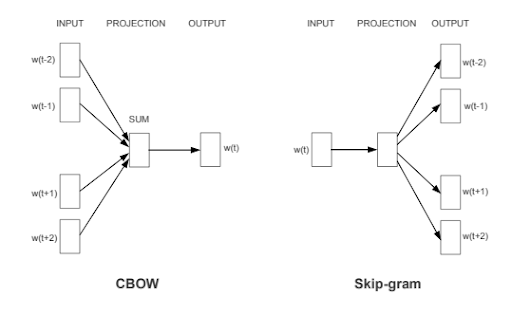
Both approaches result in a vector space that maps word-vectors close together based on contextual meaning. That means, if two word-vectors are close together, those words should have similar meaning based on their context in the corpus.

For example, using cosine similarity to analyze the vectors produced by their data, researchers were able to construct analogies like king minus man plus woman =?

The output vector most closely matched queen.

king - man + woman = queen

If this seems confusing, don’t worry. Applying and exploring word2vec is simple and will make more sense as I go through examples!

More From Eric KleppenCreate a Linux Virtual Machine on Your Computer

Dependencies and Data

The Python library Gensim makes it easy to apply word2vec, as well as several other algorithms for the primary purpose of topic modeling. Gensim is free and you can install it using Pip or Conda:

pip install --upgrade gensim

or

conda install -c conda-forge gensim

You can find the data and all of the code in my GitHub. This is the same repo as the spam email data set I used in my last article.

Import the Dependencies

from gensim.models import word2vec, FastText
import pandas as pd
import re

from sklearn.decomposition import PCA

from matplotlib import pyplot as plt
import plotly.graph_objects as go

import numpy as np

import warnings
warnings.filterwarnings('ignore')

df = pd.read_csv('emails.csv')

I start by loading the libraries and reading the .csv file using Pandas.

Exploring Word2Vec

Before playing with the email data, I want to explore word2vec with a simple example using a small vocabulary of a few sentences:

sentences = [['i', 'like', 'apple', 'pie', 'for', 'dessert'],
           ['i', 'dont', 'drive', 'fast', 'cars'],
           ['data', 'science', 'is', 'fun'],
           ['chocolate', 'is', 'my', 'favorite'],
           ['my', 'favorite', 'movie', 'is', 'predator']]

Generate Embeddings

You can see the sentences have been tokenized since I want to generate embeddings at the word level, not by sentence. Run the sentences through the word2vec model.

# train word2vec model
w2v = word2vec(sentences, min_count=1, size = 5)

print(w2v)
#word2vec(vocab=19, size=5, alpha=0.025)

Notice when constructing the model, I pass in min_count =1 and size = 5. That means it will include all words that occur ≥ one time and generate a vector with a fixed length of five. 

When printed, the model displays the count of unique vocab words, array size and learning rate (default .025).

# access vector for one word
print(w2v['chocolate'])

#[-0.04609262 -0.04943436 -0.08968851 -0.08428907  0.01970964]

#list the vocabulary words
words = list(w2v.wv.vocab)

print(words)

#or show the dictionary of vocab words
w2v.wv.vocab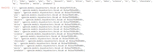

Notice that it’s possible to access the embedding for one word at a time. Also take note that you can review the words in the vocabulary a couple different ways using w2v.wv.vocab.

Visualize Embeddings

Now that you’ve created the word embeddings using word2vec, you can visualize them using a method to represent the vector in a flattened space. I am using Sci-kit Learn’s principle component analysis (PCA) functionality to flatten the word vectors to 2D space, and then I’m using Matplotlib to visualize the results.

X = w2v[w2v.wv.vocab]
pca = PCA(n_components=2)

result = pca.fit_transform(X)

# create a scatter plot of the projection
plt.scatter(result[:, 0], result[:, 1])
words = list(w2v.wv.vocab)

for i, word in enumerate(words):
   plt.annotate(word, xy=(result[i, 0], result[i, 1]))

plt.show()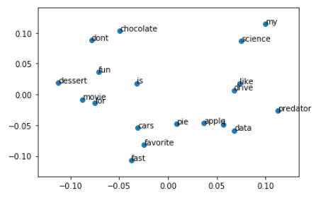

Fortunately, the corpus is tiny so it is easy to visualize; however, it’s hard to decipher any meaning from the plotted points since the model had so little information from which to learn.

Want More Matplotlib? Try This.How to Generate Subplots With Python's Matplotlib

Visualizing Email Word Embeddings

Now that I’ve walked through a simple example, it’s time to apply those skills to a larger data set. Inspect the email data by calling the dataframe head().

df.head()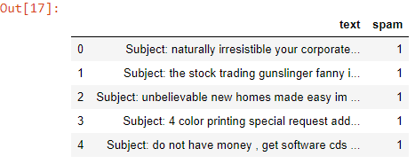

Cleaning the Data

Notice the text has not been pre-processed at all! Using a simple function and some regular expressions, cleaning the text of punctuation and special characters then setting it all to lowercase is simple.

clean_txt = []
for w in range(len(df.text)):
   desc = df['text'][w].lower()

   #remove punctuation
   desc = re.sub('[^a-zA-Z]', ' ', desc)

   #remove tags
   desc=re.sub("</?.*?>"," <> ",desc)

   #remove digits and special chars
   desc=re.sub("(\\d|\\W)+"," ",desc)
   clean_txt.append(desc)

df['clean'] = clean_txt
df.head()

Notice the clean column has been added to the dataframe and the text has been cleaned of punctuation and upper case.

Creating a Corpus and Vectors

Since I want word embeddings, we need to tokenize the text. Using a for loop, I go through the dataframe, tokenizing each clean row. After creating the corpus, I generate the word vectors by passing the corpus through word2vec.

corpus = []
for col in df.clean:
   word_list = col.split(" ")
   corpus.append(word_list)

#show first value
corpus[0:1]

#generate vectors from corpus
model = word2vec(corpus, min_count=1, size = 56)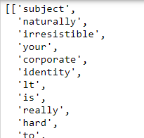

Notice the data has been tokenized and is ready to be vectorized!

More NLP on Built InA Step-by-Step NLP Machine Learning Classifier Tutorial

Visualizing Email Word Vectors

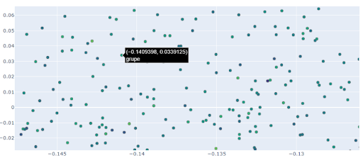
The corpus for the email data is much larger than the simple example above. Because of how many words we have, I can’t plot them like I did using Matplotlib.

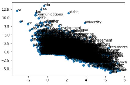
Good luck reading that! It’s time to use a different tool. Instead of Matplotlib, I’m going to use Plotly to generate an interactive visualization we can zoom in on. That will make it easier to explore the data points.

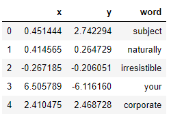
I use the PCA technique, then put the results and words into a dataframe. This will make it easier to graph and annotate in Plotly.

#pass the embeddings to PCA
X = model[model.wv.vocab]
pca = PCA(n_components=2)
result = pca.fit_transform(X)

#create df from the pca results
pca_df = pd.DataFrame(result, columns = ['x','y'])

#add the words for the hover effect
pca_df['word'] = words
pca_df.head()

Notice I add the word column to the dataframe so the word displays when hovering over the point on the graph.

Next, construct a scatter plot using Plotly Scattergl to get the best performance on large data sets. Refer to the documentation for more information about the different scatter plot options.

N = 1000000
words = list(model.wv.vocab)
fig = go.Figure(data=go.Scattergl(
   x = pca_df['x'],
   y = pca_df['y'],
   mode='markers',
   marker=dict(
       color=np.random.randn(N),
       colorscale='Viridis',
       line_width=1
   ),
   text=pca_df['word'],
   textposition="bottom center"
))

fig.show()

Notice I use NumPy to generate random numbers for the graph colors. This makes the graph a bit more visually appealing! I also set the text to the word column of the dataframe. The word appears when hovering over the data point.

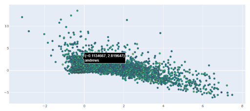
Plotly is great since it generates interactive graphs and it allows me to zoom in on the graph and inspect points more closely.

Want More? Try This Plotly Tutorial.Plotting With Plotly in Python: Data Exploration Made Easy

Analyzing and Predicting Using Word Embeddings

Beyond visualizing the embeddings, it’s possible to explore them with some code. Additionally, the models can be saved as a text file for use in future modeling. Review the Gensim documentation for the complete list of features.

#explore embeddings using cosine similarity
model.wv.most_similar('eric')

model.wv.most_similar_cosmul(positive = ['phone', 'number'], negative = ['call'])

model.wv.doesnt_match("phone number prison cell".split())

#save embeddings
file = 'email_embd.txt'
model.wv.save_word2vec_format(filename, binary = False)

Gensim uses cosine similarity to find the most similar words. 

It’s also possible to evaluate analogies and find the word that’s least similar or doesn’t match with the other words.

Using Embeddings

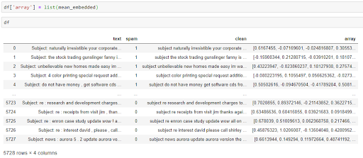
You can also use these vectors in predictive modeling. To use the embeddings, you need to map the word vectors. In order to convert a document of multiple words into a single vector using the trained model, it’s typical to take the word2vec of all words in the document, then take its mean.

mean_embedding_vectorizer = MeanEmbeddingVectorizer(model)
mean_embedded = mean_embedding_vectorizer.fit_transform(df['clean'])

To learn more about using the word2vec embeddings in predictive modeling, check out this Kaggle notebook.

Using the novel approaches available with the word2vec model, it’s easy to train very large vocabularies while achieving accurate results on machine learning tasks. Natural language processing is a complex field, but there are many libraries and tools for Python that make it easy to get started.