Understanding the Hidden Markov Model

Hidden Markov models are probabilistic frameworks where the observed data are modeled as a series of outputs generated by one of several (hidden) internal states. Both Markov and hidden Markov models are engineered to handle data that can be represented as a sequence of observations over time. 

To better understand how a hidden Markov model works, we first need to understand what a stochastic model is. 

 

What Is a Stochastic Model?

A stochastic process is a collection of random variables that are indexed by some mathematical sets. That is, each random variable of the stochastic process is uniquely associated with an element in the set. The set that is used to index the random variables is called the index set, and the set of random variables forms the state space. A stochastic process can be classified in many ways based on state space, index set, etc.

When the stochastic process is interpreted as time, if the process has a finite number of elements such as integers, numbers and natural numbers, then it is discrete time.

It’s a discrete-time process indexed at time “1,2,3,…” that takes values called states, which are observed.

• For example, if the states: (S) ={hot , cold}
• State series over time: z∈ S_T
• Weather for four days can be a sequence: {z1=hot, z2 =cold, z3 =cold, z4 =hot}

More on Machine LearningHistogram of Oriented Gradients: An Overview

 

Markov Model Assumptions

Markov models are developed based on two assumptions:

1. Limited Horizon Assumption

Probability of being in a state at a time t depend only on the state at the time (t-1).

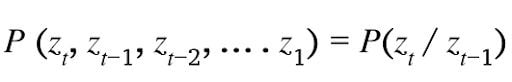
That means state at time t represents enough summary of the past to reasonably predict the future. This assumption is an order-1 Markov process. An order-k Markov process assumes conditional independence of state z_t from the states that are k + 1-time steps before it.

2. Stationary process assumption

Conditional (probability) distribution over the next state, given the current state, doesn’t change over time.

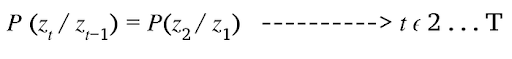
That means states keep on changing over time but the underlying process is stationary.

Notation Convention

• There is an initial state and an initial observation z_0 = s_0
• s_0: Initial probability distribution over states at time 0.
• Initial state probability: (π)
• At t=1, probability of seeing first real state z_1 is p(z_1/z_0).
• Since z0 = s0:

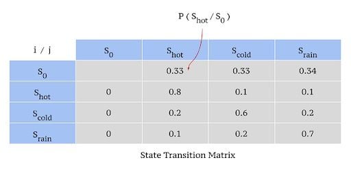
State Transition Matrix

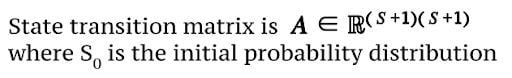
𝐀𝐢,𝐣: probability of transitioning from state i to state j at any time t.

The following chart is a state transition matrix of four states, including the initial state:

2 Questions Answered in a Markov Model

1. What is the probability of particular sequences of state z?
2. How do we estimate the parameter of state transition matrix A to maximize the likelihood of the observed sequence?

Probability of Particular Sequences in a Markov Model

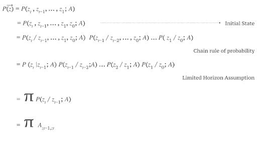
Consider the state transition matrix above. Let’s determine the probability of sequence:

{z1 = s_hot , z2 = s_cold , z3 = s_rain , z4 = s_rain , z5 = s_cold}

P(z) = P(s_hot|s_0 ) P(s_cold|s_hot) P(s_rain|s_cold) P(s_rain|s_rain) P(s_cold|s_rain)

= 0.33 x 0.1 x 0.2 x 0.7 x 0.2 = 0.000924

 

What Is a Hidden Markov Model (HMM)?

When we can’t observe the states themselves but only the result of some probability function (observation) of the states, we utilize a hidden Markov model (HMM). HMM is a statistical Markov model in which the system being modeled is assumed to be a Markov process with unobserved (hidden) states.

• Markov model: Series of (hidden) states z={z_1,z_2………….} drawn from state alphabet S ={s_1,s_2,…….𝑠_|𝑆|} where z_i belongs to S.
• Hidden Markov model: Series of observed output x = {x_1,x_2,………} drawn from an output alphabet V= {𝑣1, 𝑣2, . . , 𝑣_|𝑣|} where x_i belongs to V.

Hidden Markov Model Assumptions

A hidden Markov model is built on several assumptions, including:

1. Output Independence Assumption

Output observation is conditionally independent of all other hidden states and all other observations when given the current hidden state.

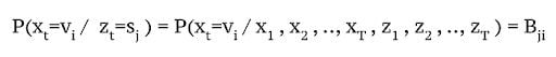
2. Emission Probability Matrix

Probability of hidden state generating output v_i given that state at the corresponding time was s_j.

 

Hidden Markov Model Example

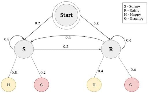
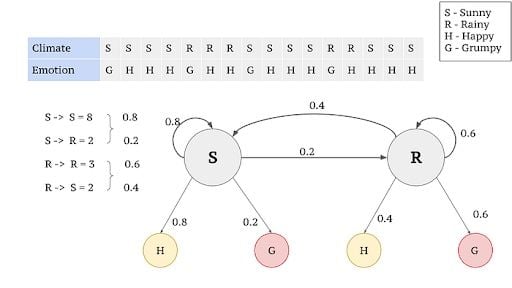
Consider the example given below, which elaborates how a person feels in different climates.

• Set of states: (S) = {Happy, Grumpy}
• Set of hidden states: (Q) = {Sunny , Rainy}
• State series over time: = z∈ S_T
• Observed states for four day: = {z1=Happy, z2= Grumpy, z3=Grumpy, z4=Happy}

The feeling that you understand from a person emoting is called the observations, since you observe them. The weather that influences the feeling of a person is called the hidden state, since you can’t observe it.

Emission Probabilities

In the above example, feelings (“Happy” or “Grumpy”) can be only observed. A person can observe that a person has an 80 percent chance to be “happy” given that the climate at the particular point of observation is sunny. Similarly there’s a 60 percent chance of a person being “grumpy” given that the climate is rainy. The 80 percent and 60 percent are emission probabilities since they deal with observations.

Transition Probabilities

When we consider the climates (hidden states) that influence the observations, there are correlations between consecutive days being sunny or alternate days being rainy. There is an 80 percent chance for the Sunny climate to be in successive days, whereas there’s a 60 percent chance for it to be rainy on consecutive days. The probabilities that explain the transition to/from hidden states are transition probabilities.

 

How Does a Hidden Markov Model Work?

A hidden Markov model answers three primary questions:

1. What is the probability of an observed sequence?
2. What is the most likely series of states to generate an observed sequence?
3. How can we learn the values for the HMMs parameters A and B given some data?

Probability of Observed Sequence

We have to add up the likelihood of the data x given every possible series of hidden states. This will lead to a complexity of O(|S|)^T. Hence, two alternate procedures were introduced to find the probability of an observed sequence.

Forward Procedure

Calculate the total probability of all the observations (from t_1) up to time t:

𝛼_𝑖 (𝑡) = 𝑃(𝑥_1 , 𝑥_2 , … , 𝑥_𝑡, 𝑧_𝑡 = 𝑠_𝑖; 𝐴, 𝐵)

Backward Procedure

Similarly calculate total probability of all the observations from final time (T) to t:

𝛽_i (t) = P(x_T , x_T-1 , …, x_t+1 , z_t= s_i ; A, B)

 

More on Machine LearningEuclidean Distance Explained

 

Hidden Markov Model Using Forward Procedure

Below is an example of a hidden Markov model using forward procedure.

• S = {hot,cold}
• v = {v1=1 ice cream ,v2=2 ice cream, v3=3 ice cream}, where V is the Number of ice creams consumed in a day.
• Example Sequence: = {x1=v2,x2=v3,x3=v1,x4=v2}

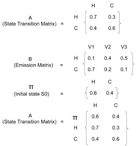
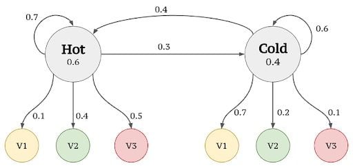
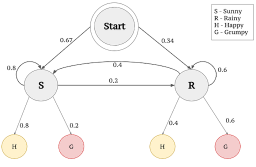
We first need to calculate the prior probabilities, that is, the probability of being hot or cold previous to any actual observation. This can be obtained from S_0 or π. From Fig.4, S_0 is provided as 0.6 and 0.4, which are the prior probabilities. Then based on Markov and HMM assumptions, we follow the steps in the figures below to calculate the probability of a given sequence.

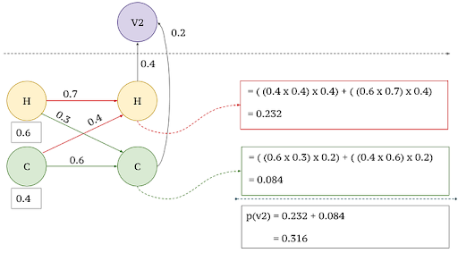
1. First Observed Output x1=v2

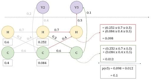
2. Observed Output x2=v3

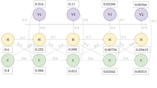
3. Observed Output x3 and x4

Similarly for x3=v1 and x4=v2, we have to simply multiply the paths that lead to v1 and v2.

4. Maximum Likelihood Assignment

For a given observed sequence of outputs𝑥 𝜖 𝑉_𝑇, we intend to find the most likely series of states𝑧 𝜖 𝑆_𝑇. We can understand this with an example found below.

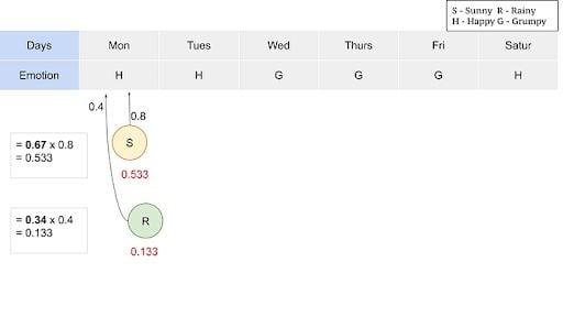
The Viterbi algorithm is a dynamic programming algorithm similar to the forward procedure which is often used to find maximum likelihood. Instead of tracking the total probability of generating the observations, it tracks the maximum probability and the corresponding state sequence.

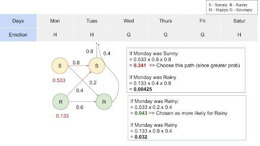
Consider the sequence of emotions: H,H,G,G,G,H for six consecutive days. Using the Viterbi algorithm we will find out the more likelihood of the series.

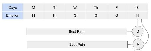
There will be several paths that will lead to sunny on Saturday, and many paths that lead to rainy on Saturday. Here, we intend to identify the best path to sunny or rainy Saturday and multiply with the transition emission probability of “Happy,” since Saturday makes the person feel “Happy.”

Let’s consider a sunny Saturday. The previous day, Friday, can be sunny or rainy. Then we need to know the best path up to Friday, and then multiply with emission probabilities that lead to a grumpy feeling. Iteratively, we need to figure out the best path at each day ending up in more likelihood of the series of days.

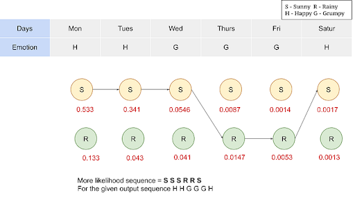
 The algorithm leaves you with maximum likelihood values and we now can produce the sequence with a maximum likelihood for a given output sequence.

5. Learn the Values for the HMMs Parameters A and B

Learning in HMMs involves estimating the state transition probabilities A and the output emission probabilities B that make an observed sequence most likely. Expectation-Maximization algorithms are used for this purpose. An algorithm known as the Baum-Welch algorithm falls under this category and uses the forward algorithm. It’s commonly used.

This article comprehensively describes Markov and hidden Markov models. Its main intent has been  to provide an explanation with an example to find the probability of a given sequence and maximum likelihood for HMM which is often questionable in examinations, too. 

Frequently Asked Questions