

Histogram of oriented gradients (HOG) is a feature descriptor like the Canny edge detector and scale invariant and feature transform (SIFT). It’s used in computer vision and image processing for the purpose of object detection. The technique counts occurrences of gradient orientation in the localized portion of an image.
What Is the Histogram of Oriented Gradients Method?
The histogram of oriented gradients method is a feature descriptor technique used in computer vision and image processing for object detection. It focuses on the shape of an object, counting the occurrences of gradient orientation in each local region. It then generates a histogram using the magnitude and orientation of the gradient.
Histogram of oriented gradients method is also quite similar to edge orientation histograms and SIFT. The HOG descriptor focuses on the structure or the shape of an object. It’s better than any edge descriptor as it uses magnitude as well as the angle of the gradient to compute the features. For the regions of the image, it generates histograms using the magnitude and orientations of the gradient.
How to Calculate the Histogram of Oriented Gradients Features
Below are the 10 steps in the histogram of oriented gradients
1. Prepare the Input Image
Take the input of the image you want to calculate HOG features. Resize the image into an image of 128x64 pixels (128 pixels height and 64 pixels width). In a research paper on HOG, the authors used this dimension in the paper and suggested it as their primary aim with this type of detection was to obtain better results on the task of pedestrian detection.
As the authors of this paper were obtaining exceptionally perfect results on the MIT pedestrian database, they decided to produce a new and significantly more challenging data set called the ‘INRIA’ data set, containing 1805 (128x64) images of humans cropped from a varied set of personal photos.

2. Calculate the Gradient of the Image
The gradient of the image is calculated. The gradient is obtained by combining magnitude and angle from the image. Consider a block of 3x3 pixels, first Gx and Gy is calculated for each pixel using the formula below for each pixel value.

After calculating Gx and Gy, the magnitude and angle of each pixel is calculated using the formula mentioned below.


3. Divide the Gradient Matrices to Form a Block
After obtaining the gradient of each pixel, the gradient matrices (magnitude and angle matrix) are divided into 8x8 cells to form a block. For each block, a nine-point histogram is calculated. A nine-point histogram develops a histogram with nine bins and each bin has an angle range of 20 degrees. Figure 8 represents a nine-bin histogram in which the values are allocated after calculations. Each of these nine-point histograms can be plotted as histograms with bins outputting the intensity of the gradient in that bin.
A block contains 64 different values. The following calculation will be performed for all 64 values of magnitude and gradient:

Each Jth bin, bin will have boundaries from:

The value of the center of each bin will be:


This one single histogram will be unique for one 8x8 block made up of 64 cells. All 64 cells will add their Vj and Vj+1 value to the jth and (j+1)th index of the array respectively.
4. Calculate the Jth Bin
For each cell in a block, we will first calculate the jth bin and then the value that will be provided to the jth and (j+1)th bin respectively. The value is given by the following formulas:

5. Calculate the Arrays for Each Pixel
An array is taken as a bin for a block and values of Vj and Vj+1 is appended in the array at the index of jth and (j+1)th bin calculated for each pixel.
6. Histogram Computation Is Finished for Each Block
The resultant matrix after the above calculations will have the shape of 16x8x9.
7. Club Together the Blocks
Once histogram computation is over for all blocks, four blocks from the nine-point histogram matrix are clubbed together to form a new block (2x2). This clubbing is done in an overlapping manner with a stride of eight pixels. For all four cells in a block, we concatenate all the nine-point histograms for each constituent cell to form a 36 feature vector.


8. Calculate the L2 Norm
Values of fb for each block is normalized by the L2 norm:

Where ε is a small value added to the square of fb in order to avoid zero division error. In code value taken is 1e-05. (Image by author)
9. Normalize the Value
To normalize, the value of k is first calculated by the following formula:

10. Obtain the HOG Features
This normalization is done to reduce the effect of changes in contrast between images of the same object. From each block, a 36-point feature vector is collected. In the horizontal direction there are 7 blocks and in the vertical direction there are 15 blocks. So the total length of HOG features will be : 7 x 15 x 36 = 3780. HOG features of the selected image are obtained.
Histogram of Oriented Gradients Features From Scratch in Python
Here are the steps to calculating the histogram of oriented gradients features in Python.
1. Import the Libraries and Image
import matplotlib.pyplot as plt
from skimage import io
from skimage import color
from skimage.transform import resize
import math
from skimage.feature import hog
import numpy as np


img = resize(color.rgb2gray(io.imread("B.jpg")), (128, 64))
2. Visualization of the Image
plt.figure(figsize=(15, 8))
plt.imshow(img, cmap="gray")
plt.axis("off")
plt.show()

img = np.array(img)
3. Calculate the Gradient and Angle of the Image
mag = []
theta = []
for i in range(128):
  magnitudeArray = []
  angleArray = []
  for j in range(64):
    # Condition for axis 0
    if j-1 <= 0 or j+1 >= 64:
      if j-1 <= 0:
        # Condition if first element
        Gx = img[i][j+1] - 0
      elif j + 1 >= len(img[0]):
        Gx = 0 - img[i][j-1]
    # Condition for first element
    else:
      Gx = img[i][j+1] - img[i][j-1]

    # Condition for axis 1
    if i-1 <= 0 or i+1 >= 128:
      if i-1 <= 0:
        Gy = 0 - img[i+1][j]
      elif i +1 >= 128:
        Gy = img[i-1][j] - 0
    else:
      Gy = img[i-1][j] - img[i+1][j]

    # Calculating magnitude
    magnitude = math.sqrt(pow(Gx, 2) + pow(Gy, 2))
    magnitudeArray.append(round(magnitude, 9))

    # Calculating angle
    if Gx == 0:
      angle = math.degrees(0.0)
    else:
      angle = math.degrees(abs(math.atan(Gy / Gx)))
    angleArray.append(round(angle, 9))
  mag.append(magnitudeArray)
  theta.append(angleArray)
mag = np.array(mag)
theta = np.array(theta)
4. Visualization of the Image Magnitude
plt.figure(figsize=(15, 8))
plt.imshow(mag, cmap="gray")
plt.axis("off")
plt.show()

5. Visualization of the Image Angle
plt.figure(figsize=(15, 8))
plt.imshow(theta, cmap="gray")
plt.axis("off")
plt.show()

number_of_bins = 9
step_size = 180 / number_of_bins
6. Function to Calculate the Jth Bin
def calculate_j(angle):
  temp = (angle / step_size) - 0.5
  j = math.floor(temp)
  return j
7. Function to Calculate the Center Value of Jth Bin
def calculate_Cj(j):
  Cj = step_size * (j + 0.5)
  return round(Cj, 9)
8. Function to Calculate the Value of Jth Bin
def calculate_value_j(magnitude, angle, j):
  Cj = calculate_Cj(j+1)
  Vj = magnitude * ((Cj - angle) / step_size)
  return round(Vj, 9)
9. Create a 9-Point Histogram for 8x8 Cells
histogram_points_nine = []
for i in range(0, 128, 8):
  temp = []
  for j in range(0, 64, 8):
    magnitude_values = [[mag[i][x] for x in range(j, j+8)] for i in range(i,i+8)]
    angle_values = [[theta[i][x] for x in range(j, j+8)] for i in range(i, i+8)]
    for k in range(len(magnitude_values)):
      for l in range(len(magnitude_values[0])):
        bins = [0.0 for _ in range(number_of_bins)]
        value_j = calculate_j(angle_values[k][l])
        Vj = calculate_value_j(magnitude_values[k][l], angle_values[k][l], value_j)
        Vj_1 = magnitude_values[k][l] - Vj
        bins[value_j]+=Vj
        bins[value_j+1]+=Vj_1
        bins = [round(x, 9) for x in bins]
    temp.append(bins)
  histogram_points_nine.append(temp)
print(len(histogram_points_nine))
print(len(histogram_points_nine[0]))
print(len(histogram_points_nine[0][0]))

16
8
9
10. Create a Histogram of Oriented Gradient Feature Vector for 9-Point Histogram With 2x2 Blocks
One block is made up by 8x8 cells.
epsilon = 1e-05
feature_vectors = []
for i in range(0, len(histogram_points_nine) - 1, 1):
  temp = []
  for j in range(0, len(histogram_points_nine[0]) - 1, 1):
    values = [[histogram_points_nine[i][x] for x in range(j, j+2)] for i in range(i, i+2)]
    final_vector = []
    for k in values:
      for l in k:
        for m in l:
          final_vector.append(m)
    k = round(math.sqrt(sum([pow(x, 2) for x in final_vector])), 9)
    final_vector = [round(x/(k + epsilon), 9) for x in final_vector]
    temp.append(final_vector)
  feature_vectors.append(temp)
print(len(feature_vectors))
print(len(feature_vectors[0]))
print(len(feature_vectors[0][0]))
15
7
36
11. Number of Histogram of Oriented Gradient Features Obtained
print(f'Number of HOG features = {len(feature_vectors) * len(feature_vectors[0]) * len(feature_vectors[0][0])}')

Number of HOG features = 3780
Histogram of Oriented Gradient Features Using Skimage Library in Python
Follow these steps to calculate the histogram of oriented gradient features using Python’s SKimage library.
1. Import the Libraries
from skimage.io import imread
from skimage.transform import resize
from skimage.feature import hog
from skimage import exposure
import matplotlib.pyplot as plt
2. Read the Image
img = imread('B.jpg')
plt.axis("off")
plt.imshow(img)
print(img.shape)

(781, 794, 3)

3. Resize the Image
resized_img = resize(img, (128*4, 64*4))
plt.axis("off")
plt.imshow(resized_img)
print(resized_img.shape)

(512, 256, 3)
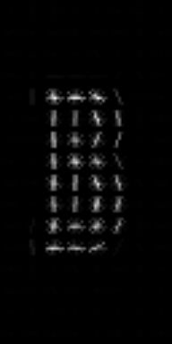
4. Create and Visualize the Histogram of Oriented Gradient Features
fd, hog_image = hog(resized_img, orientations=9, pixels_per_cell=(8, 8),
                	cells_per_block=(2, 2), visualize=True, multichannel=True)
plt.axis("off")
plt.imshow(hog_image, cmap="gray")
plt.show()


