

Scientists often encounter extraordinarily large data sets. This happens for a very good reason: more data provides a more thorough understanding of the phenomenon they’re studying. But it also creates a problem. As data sets get larger they become harder to understand and use.
One solution is learning how to automatically split your data sets into separate files so each data file becomes a manageable amount of information to explain a single of the phenomenon. The data becomes much easier to work with and, by splitting your data sets automatically, you make your work much easier with very little effort.
What Should I Expect?
In this portion of the tutorial we’ll cover the process of splitting a data set containing results from multiple laboratory tests into individual files. Those files will each contain the results of a single test and will have descriptive file names stating what data is contained within them.
Let’s focus on a real life problem often encountered in science and engineering. To understand the foundational concepts, make sure to check out part one of this series. If you want to go even deeper and leave the tutorial with confidence in your skills and new tools, you can download the companion data set, which will allow you to test your code and check your results to ensure you’re learning this process correctly.
Steps to Split Your Data Set
- Import Python packages.
- Identify the end of each test.
- Save each test as a new file.
- Run the script to confirm each new file holds the relevant data.
Let’s get started. First, import the Python packages that will enable the data analysis process.
How Do I Import Packages in Python?
Each Python script needs to start with statements importing the required packages and capabilities. In this data file splitting script we’ll need:
-
Pandas: This package is the premier option for data analysis in Python. Pandas will allow you to read your data into DataFrames (essentially tables) and provides a vast array of tools for manipulating that data.
-
os: This Python package enables you to use commands from the computer’s operating system, which impact the computer outside of the data analysis process. In this case we’ll use it to create new folders.
-
Bokeh: Bokeh is an interactive plotting tool in Python. It enables you to write code that automatically generates plots while analyzing your data and gives options for the user to interact with them.
For our purposes, we’ll pull in the entirety of both Pandas and os, but only specific functions from Bokeh. To do that, add the following code to the start of your program.
import pandas as pd
import os
from bokeh.plotting import figure, save, gridplot, output_file,   ColumnDataSource
from bokeh.models import HoverTool
You can see those four lines importing the stated packages. Note the line to import Pandas also specifies we’ve imported Pandas as pd, meaning we can refer to Pandas as “pd” in the rest of the code. Also note that ColumnDataSource is on the code line that starts with from bokeh.plotting.
Now that we’ve imported our packages, the next step is to read the necessary data so the script can work with it.
How Do I Read the Data Files?
Pandas has a fantastic tool for importing data sets: the read_csv function. In order to read a file, you call the pandas.read_csv function, specify the location of the file and set it to a variable. (There are several other modifiers you can use to customize the import if desired, but we won’t be using them here.)
We’ll use this command to import two files. The first file is the data set itself. If you downloaded the companion data set, it’s titled COP_HPWH_f_Tamb&Tavg.csv.
If we imagine that you saved the file in the folder C:\Users\YourName\Documents\AutomatedDataAnalysis, then we can import the data with the following code. (You’ll need to change “YourName” to your user profile name.)
Data = pd.read_csv(r’C:\Users\YourName\Documents\AutomatedDataAnalysis\COP_HPWH_f_Tamb&Tavg.csv’)
Executing that code will save the data set to the variable “Data.” This means you can use all the Pandas data analysis capabilities on the data set by referencing Data.
The second file we’ll need is a table describing the tests contained in the file. For the sake of practice, it’s helpful if you create the table yourself.
The data set contains the results from three tests, with different ambient temperatures (the temperature of air around the tested device). To create this data set, generate a table with the following information and save it as “Test_Plan.csv” in the same folder as your data set.
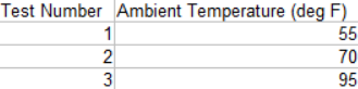
Later you’ll reference the names of the columns, so it’s important to make sure you use the same text as in the example data.
Now that you’ve created and saved the table, you can read it into Python by writing:
Test_Plan = pd.read_csv(r’C:\Users\YourName\Documents\AutomatedDataAnalysis\Test_Plan.csv’)Next you’ll identify the rows where each test ends and the next test begins.
How Do I Identify Where Each Test Ends?
First things first: you’ll need some knowledge about the tests themselves. Think about the project’s test procedure and identify a condition that would indicate that one test is ending.
In this case we’re analyzing data from tests studying heat pump water heaters (HPWH), which use electricity to heat water. Since we’re looking at how much electricity the HPWH consumes to heat the water, we can know it’s consuming electricity during each test. This means that each test ends when the device stops using electricity.
We need to identify rows where the device stops using electricity, which we can do by subtracting the electricity consumption in each row from the electricity consumption in the previous row. If the result is negative, that means the HPWH is consuming less electricity than it previously had, which indicates the test ended.
We accomplish this by using the .shift() function on our data set. This function does what it sounds like; it shifts the data by a specified number of rows. We can use .shift() to create a new row in the data frame that contains electricity consumption, P_Elec (W), data that has been shifted by one row. We can do this with the following line of code:
Data[‘P_Elec_Shift (W)’] = Data[‘P_Elec (W)’].shift(periods = -1)This leads to two different columns in the data frame describing the HPWHs electricity consumption. P_Elec (W) states the electricity consumption, in Watts, in each row. P_Elec_Shift (W) states the electricity consumption, in Watts, of the next row. If we subtract P_Elec (W) from P_Elec_Shift (W), rows with negative values will indicate the HPWH has stopped heating. Let’s use the following code:
Data[‘P_Elec_Shift (W)’] = Data[‘P_Elec_Shift (W)’] — Data[‘P_Elec (W)’]At this point we have a data frame with a row that contains zero in every row except rows where each test ended. We can use that information to create a list that tells us when each test ended. We’ll call that list End_Of_Tests, to clearly signify the information contained within it. We’ll then use the .index.tolist() function to populate that list. We can do this with the following code:
End_Of_Tests = []

End_Of_Tests = End_Of_Tests + Data[Data[‘P_Elec_Shift (W)’] < 0].index.tolist()
The first line creates the empty list End_Of_Tests. While it originally holds no data, it’s ready to accept data from other commands. The second line adds data to End_Of_Tests. It says to look through Data to identify rows where P_Elec_Shift (W) is negative, identify the index of those rows, and add them to the End_Of_Tests list.
Now that we’ve identified the rows that correspond to the end of each test we can split the data set into separate data sets, one for each test.
How Do I Split the Data File?
We can split the data file into more manageable files using the following steps:
- Repeat the process once for each test. This means we need to iterate through it once for each entry in End_Of_Tests.
- Create a new data frame that is a subset of the original data frame containing only data from a single test.
- Use the conditions of the test to identify the test in the test plan that this data represents.
- Save the data to a new file with a file name that states what data is contained in the file.
1. IteratE through End_Of_Tests
We accomplish this first step with a simple for loop that iterates through the End_Of_Tests list. You can do this with the following code:
for i in range(len(End_Of_Tests)):This creates a loop that runs x times, where x is the number of rows in End_Of_Tests/the number of tests contained in the file. Note that i will be an increasing integer (0, 1, 2, and so on) and can be used as an index. Also note that we now have an active for loop, so all future code will need to be indented until we leave the for loop.
2. CreatE New Data Frames With Subsets of the Data
We do this by using the values of End_Of_Tests to identify the rows of Data corresponding to each test. In the first test, this means we need to select the data between the first row and the first value in End_Of_Tests. In the second test, this means we need to select the data between the first value in End_Of_Tests and the second value in End_Of_Tests. (We’d do the same for the third and so on if we have more than three tests in this data set.)
The difference in handling between the first test (which starts at hard-coded row zero) and the future tests (which start at an entry in End_Of_Tests) requires an if statement that changes the code based on whether or not we’re pulling out the first test.
The code then needs to use the End_Of_Test values to identify the section of Data that we want, and save it to a new data frame.
We do this with the following code:
if i == 0:
   File_SingleTest = Data[0:End_Of_Tests[i]]
else:
   File_SingleTest = Data[End_Of_Tests[i-1]:End_Of_Tests[i]]
The first line checks to see if this code is being executed for the first time. If it is, that means it’s the first time through the loop and we’re extracting the first test. If this is the code’s first time through the loop, the code pulls the first row of Data (Index 0) through the first entry in End_Of_Tests (Denoted with End_Of_Tests[i], which is currently End_Of_Tests[0]) and stores it in a new data frame called File_SingleTest.
If this isn’t the first time through the code, that means we need to extract data from a test that’s not the first. In that case we extract data from when the previous test ended (End_Of_Tests[i-1]) to when the current test ends (End_Of_Tests[i]) and save it to File_SingleTest.
Note that the data is always saved to File_SingleTest. This means that the data frame containing data from a single test will always be overwritten in the next iteration. It’s important to save the data before that happens!
3. Identify the Conditions of Each Test
Now we have a data frame containing the data of a specific test, but which test is it? We need to read the data to understand what happens in that test and compare it to the specifications in the test plan. In that way we can identify which test is in the data frame and give the data frame a descriptive name.
Looking at the test plan, we see the ambient temperature changes in each test. Test number one has an ambient temperature of 55 degrees Fahrenheit, test two has 70 degrees Fahrenheit, and test three has 95 degrees Fahrenheit. This means that ambient temperature is our descriptor here.
We can identify the ambient temperature during a test with the following code:
Temperature_Ambient = File_SingleTest[‘T_Amb (deg F)’][-50:].mean()This line reads the last 50 entries ([-50:]) of the column representing ambient temperature (‘T_Amb (deg F)’) in the File_SingleTest data frame and calculates the average (.mean()). The code then stores that value in Temperature_Ambient. This means we have the ambient temperature for the last few minutes of the test stored in a variable.
The second step is to compare this value to the test plan and identify which test the code performed. This is important because no test data will ever be perfect and the average ambient temperature will not perfectly match the specification in the test plan.
For example, a test with a 55 degree ambient temperature specified may actually have a 53.95 degree ambient temperature. Identifying the corresponding test makes file management easier.
We can identify the corresponding test by both calculating the difference between the average temperature in the test and the ambient temperature called for in each test, and identifying the test with the minimum difference. Do this with the following two lines of code:
Test_Plan[‘Error_Temperature_Ambient’] = abs(Test_Plan[‘Ambient Temperature (deg F)’] — Temperature_Ambient)

Temperature_Ambient = Test_Plan.loc[Test_Plan[‘Error_Temperature_Ambient’].idxmin(), ‘Ambient Temperature (deg F)’]
The first line adds a new column to the Test_Plan data frame that states the absolute value of the difference between the ambient temperature called for in that test and the average ambient temperature in the active test. The second line uses the .loc() and .idxmin() functions to identify the ambient temperature specified in the test with the least error and set that ambient temperature to our Temperature_Ambient variable.
Now we’re ready to save the data in a new file.
4. SavE the Data to a New File
With a data frame containing the results from a single test, and knowledge of the conditions of that test, we can now save the results to a new file.
First, ensure the folder in which we want to save the data actually exists. We could do that manually, but this is an article about automating things! Let’s program the script to do it for us.
Let’s say we want the data to be stored in the file C:\Users\YourName\Documents\AutomatingDataAnalysis\Files_IndividualTests. To make sure that folder exists we can use the following code:
Folder = ‘C:\Users\YourName\Documents\AutomatingDataAnalysis\Files_IndividualTests’

if not os.path.exists(Folder):

   os.makedirs(Folder)
The first line sets the path of our desired folder to the variable Folder. The second line uses the os function .path.exists() to check and see if that folder exists. If it doesn’t exist, it executes the third line of code to create the folder.
Once the folder exists, we can use the same approach to save the data file into that folder. We specify the file name we want to use, using variables to contain data about the ambient temperature, and use the pandas.to_csv() function to save the file where we desire. You can do this with the following code:
Filename_SingleTest = “\PerformanceMap_HPWH_” + str(int(Temperature_Ambient)) + “.csv”

File_SingleTest.to_csv(Folder + Filename_SingleTest, index = False)
The first line creates the file name we want to use. It descriptively states it’s a file containing data from testing used to create a performance map of a HPWH. The second part is more important. It takes the ambient temperature that we identified in the test plan as a variable, converts it to an integer, converts it to a string and adds it to the file name. Now the file name contains the conditions of the test and tells you exactly what the file contains before you even open it.
The second line does the grunt work. It combines the folder specified previously with the file name for the current data frame and saves it. Note it also removes the index because saving that isn’t important and helps keep files cleaner.
What’s the Final Step?
Now you’re at the fun part of writing this script: you get to run it! You also get to watch the program generate the results you need for you.
(Note this process is a bit overkill in this instance. The companion data set has results from three fabricated tests. It wouldn’t be very difficult, time consuming or tedious to do this manually in a project with three tests. But what if you had 1,000 tests? That’s when this process becomes extremely valuable.)
How Do I Check my Results?
Checking your results is a two-step process.
First, ensure you got the right files as outputs. To do that, you compare the files in your new folder to the tests called for in the test plan. There should be one file for each test, with the conditions in the file name matching the conditions called for in the test plan.
In this process, you should see the following files in your folder:
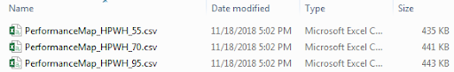
Notice how there are three files in that folder, and three tests specified in the test plan. Also notice how the test plan calls for tests at 55, 70 and 95 degrees, and those three temperatures are specified in the three file names. So far, it looks like everything worked correctly.
Next, examine the data contained in each file. The easiest way to do that is by plotting the data and visually examining it (we’ll discuss ways to automate this process later).
A quick check you can do is to create a plot showing the ambient temperature from each data file, which you can do with Bokeh.
First, we need to create a new column in the data frame that gives us the test time in user-friendly terms (minutes since the test started). We do this by adding the following line to our program (if we assume that the time between measurements is five seconds):
File_SingleTest[‘Time_SinceStart (min)’] = File_SingleTest.index * 10./60.That gives us a user-friendly time interval to use as the x-axis in our plot. Then we can use Bokeh to create and save the plot. We do that with the following code:
p1 = figure(width=800, height=400, x_axis_label=’Time (min)’, y_axis_label = ‘Temperature (deg F)’)

p1.circle(File_SingleTest[‘Time_SinceStart (min), File_SingleTest[‘T_Amb (deg F)’], legend=’Ambient Temperature’, color = ‘red’, source = source_temps)
The first line creates a figure called p1 and specifies both the size and axis labels for the plot. The second line adds red circles to the plot with the x-values specified by Time_Since Start (min) and the y-values specified by T_Amb (deg F). The first line also states the legend reading should be Ambient Temperature.
You can save the plot using the gridplot and output file features.
p=gridplot([[p1]])

output_file(Folder + '\PerformanceMap_HPWH_T_Amb=’ + str(int(Temperature_Ambient)) + ‘.html’, title = ‘Temperatures’)

save(p)
Pro tip: Bokeh has a handy feature called gridplot that enables you to store multiple plots in a single file. This makes it convenient to look at related plots next to each other and compare the data in them. This feature is not necessary for this tutorial, so we only entered our current plot (p1) in the grid. But you should know about it in case you want it in the future.
The second line specifies where the file should be saved. It goes in the same folder where we saved the .csv files of the data, and uses the same file name convention as before. The difference is that the data was saved in .csv files and this is saved in an .html file.
The third line finally saves the data.
If you re-run the code, you’ll see the same .csv files in your results folder. Additionally, you’ll now find new .html files. These .html files contain the data sets’ plots.
What would you expect to see if you open the plots?
First, you’d expect the ambient temperature recorded during the tests to be similar to the values specified in the test plan and file name. The tests at 55 degrees should have ambient temperatures around 55 degrees, and so on.
Second, with this being real world data you shouldn’t expect it to be perfect. Some values will be 54.5, others will be 55.2 and so on. Don’t freak out about that.
Third, you should expect to see the temperature adjusting at the start of the test. The original values will be at the temperature from the previous test, then the lab will need to gradually change the temperature to the new setting.
If we open the plot from the 55 degree test, we should see exactly that. Here’s what your result should look like:
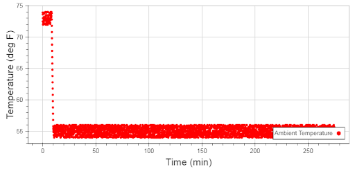
Notice how the temperature starts at 75 degrees, then rapidly decreases to 55 degrees, as expected. Notice how the average temperature throughout the test is clearly 55 degrees, also as expected. Finally, notice how the data bounces around 55 degrees...just as we expected.
This file implies our code performed the test correctly and the data file split as we hoped.
What’s Next?
Now that the overwhelmingly large data file is split into three separate files, one for each test, we can begin to make use of those data files. The next step is to check the process of the data files so we can perform our analysis. When we finish the analysis, we can then check the results to ensure that the test and calculations are correct.
* * *
This multi-part tutorial will teach you all the skills you need to automate your laboratory data analysis and develop a performance map of heat pump water heaters. You can find the rest of the series here:
Need to Automate Your Data Analysis? Here’s How to Get Started.
These Python Scripts Will Automate Your Data Analysis
How to Check Your Data Analysis for Errors
Don't DIY. Write Python Scripts to Check Data Quality for You.


