Dynamic time warping (DTW) is a way to compare two temporal sequences that do not perfectly sync up. It is a method to calculate the optimal matching between two sequences. DTW is useful in many domains such as speech recognition, data mining and financial markets. It’s commonly used in data mining to measure the distance between two time series.
What Is Dynamic Time Warping?
Dynamic time warping (DTW) is a way of comparing two temporal sequences that don’t perfectly sync up through mathematics. The process is commonly used in data mining to measure the distance between two time series. It’s also a useful method in fields like financial markets and speech recognition.
We will go over the mathematics behind DTW. Then, we’ll explore two illustrative examples to better understand the concept.
How to Form Dynamic Time Warping
Let’s assume we have two sequences like the following:
?=?[1], ?[2], …, x[i], …, x[n]Y=y[1], y[2], …, y[j], …, y[m]
The sequences X and Y can be arranged to form an ?-by-? grid, where each point (?, j) is the alignment between x[?] and y[?].
A warping path W maps the elements of X and Y to minimize the distance between them. W is a sequence of grid points (?, ?). We will see an example of the warping path later.
Dynamic Time Warping Distance and Warping Path
The optimal path to (?_?, ?_?) can be computed by:

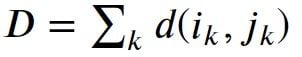
In the above equation, ? is the Euclidean distance. Then, the overall path cost can be calculated as:
Dynamic Time Warping Constraints
The warping path is found using a dynamic programming approach to align two sequences. Going through all possible paths is “combinatorially explosive,”according to a research article titled “Using Dynamic Time Warping to Find Patterns in Time Series.” Therefore, it’s important to limit the number of possible warping paths for efficiency purposes. The following constraints are outlined:
- Boundary condition: This constraint ensures that the warping path begins with the start points of both signals and terminates with their endpoints.

- Monotonicity condition: This constraint preserves the time-order of points so that it doesn’t go back in time.
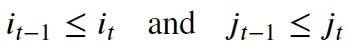
- Continuity (step-size) condition: This constraint limits the path transitions to adjacent points in time so that it doesn’t jump in time.

In addition to the above three constraints, there are other, less frequent conditions for an allowable warping path:
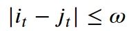
- Warping window condition: Allowable points can be restricted to fall within a given warping window of width ? (a positive integer).
- Slope condition: The warping path can be constrained by restricting the slope, and consequently, avoid extreme movements in one direction.
An acceptable warping path has combinations of chess king moves that are:
- Horizontal moves: (?, ?) → (?, ?+1)
- Vertical moves: (?, ?) → (?+1, ?)
- Diagonal moves: (?, ?) → (?+1, ?+1)
How to Implement Dynamic Time Warping
Let’s import our Python packages.
import pandas as pd
import numpy as np

# Plotting Packages
import matplotlib.pyplot as plt
import seaborn as sbn

# Configuring Matplotlib
import matplotlib as mpl
mpl.rcParams['figure.dpi'] = 300
savefig_options = dict(format="png", dpi=300, bbox_inches="tight")

# Computation packages
from scipy.spatial.distance import euclidean
from fastdtw import fastdtw
Then, we’ll define a method to compute the accumulated cost matrix D for the warp path. The cost matrix uses the Euclidean distance to calculate the distance between every two points. The methods to compute the Euclidean distance matrix and accumulated cost matrix are defined below:
def compute_euclidean_distance_matrix(x, y) -> np.array:
    """Calculate distance matrix
    This method calculates the pairwise Euclidean distance between two sequences.
    The sequences can have different lengths.
    """
    dist = np.zeros((len(y), len(x)))
    for i in range(len(y)):
        for j in range(len(x)):
            dist[i,j] = (x[j]-y[i])**2
    return dist
def compute_accumulated_cost_matrix(x, y) -> np.array:
"""Compute accumulated cost matrix for warp path using Euclidean distance
"""
distances = compute_euclidean_distance_matrix(x, y)
# Initialization
cost = np.zeros((len(y), len(x)))
cost[0,0] = distances[0,0]
for i in range(1, len(y)):
cost[i, 0] = distances[i, 0] + cost[i-1, 0]
for j in range(1, len(x)):
cost[0, j] = distances[0, j] + cost[0, j-1]
# Accumulated warp path cost
for i in range(1, len(y)):
for j in range(1, len(x)):
cost[i, j] = min(
cost[i-1, j], # insertion
cost[i, j-1], # deletion
cost[i-1, j-1] # match
) + distances[i, j]
return cost
Can You Calculate Euclidean Distance With Different Lengths?
In this example, we have two sequences x and y with different lengths.
# Create two sequences
x = [3, 1, 2, 2, 1]
y = [2, 0, 0, 3, 3, 1, 0]
We cannot calculate the Euclidean distance between x and y since they don’t have equal lengths.
How to Find Dynamic Time Warping Distance and Warp Path
Many Python packages calculate the DTW by just providing the sequences and the type of distance, which is usually Euclidean. Here, we use a popular Python implementation of DTW called FastDTW, which is an approximate DTW algorithm with lower time and memory complexities, according to a Florida Institute of Technology research article.
dtw_distance, warp_path = fastdtw(x, y, dist=euclidean)Note that we are using SciPy’s distance function Euclidean that we imported earlier. For a better understanding of the warp path, let’s first compute the accumulated cost matrix and then visualize the path on a grid. The following code will plot a heat map of the accumulated cost matrix.
cost_matrix = compute_accumulated_cost_matrix(x, y)
fig, ax = plt.subplots(figsize=(12, 8))
ax = sbn.heatmap(cost_matrix, annot=True, square=True, linewidths=0.1, cmap="YlGnBu", ax=ax)
ax.invert_yaxis()

# Get the warp path in x and y directions
path_x = [p[0] for p in warp_path]
path_y = [p[1] for p in warp_path]

# Align the path from the center of each cell
path_xx = [x+0.5 for x in path_x]
path_yy = [y+0.5 for y in path_y]

ax.plot(path_xx, path_yy, color='blue', linewidth=3, alpha=0.2)

fig.savefig("ex1_heatmap.png", **savefig_options)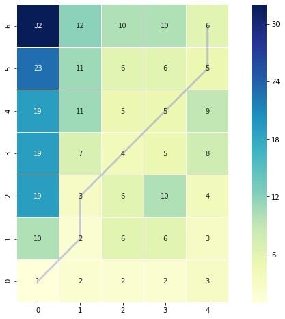
The color bar shows the cost of each point in the grid. The warp path, or blue line, is going through the lowest cost on the grid. Let’s print these two variables to see the DTW distance and the warping path.
>>> DTW distance:  6.0
>>> Warp path: [(0, 0), (1, 1), (1, 2), (2, 3), (3, 4), (4, 5), (4, 6)]
The warping path starts at point (0, 0) and ends at (4, 6) by six moves. Let’s also calculate the accumulated cost using the functions we defined earlier and compare the values with the heat map.
cost_matrix = compute_accumulated_cost_matrix(x, y)
print(np.flipud(cost_matrix)) # Flipping the cost matrix for easier comparison with heatmap values!
>>> [[32. 12. 10. 10.  6.]
     [23. 11.  6.  6.  5.]
     [19. 11.  5.  5.  9.]
     [19.  7.  4.  5.  8.]
     [19.  3.  6. 10.  4.]
     [10.  2.  6.  6.  3.]
     [ 1.  2.  2.  2.  3.]]
The cost matrix printed above has similar values to the heat map.
Now let’s plot the two sequences and connect the mapping points. The code to plot the DTW distance between x and y is given below.
fig, ax = plt.subplots(figsize=(14, 10))

# Remove the border and axes ticks
fig.patch.set_visible(False)
ax.axis('off')

for [map_x, map_y] in warp_path:
    ax.plot([map_x, map_y], [x[map_x], y[map_y]], '--k', linewidth=4)

ax.plot(x, '-ro', label='x', linewidth=4, markersize=20, markerfacecolor='lightcoral', markeredgecolor='lightcoral')
ax.plot(y, '-bo', label='y', linewidth=4, markersize=20, markerfacecolor='skyblue', markeredgecolor='skyblue')
ax.set_title("DTW Distance", fontsize=28, fontweight="bold")

fig.savefig("ex1_dtw_distance.png", **savefig_options)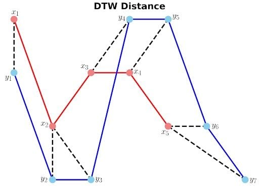
Calculating the Dynamic Time Warping Distance Between Two Sinusoidal Signals
In this example, we will use two sinusoidal signals and calculate the DTW distance between them to see how they will be matched.
time1 = np.linspace(start=0, stop=1, num=50)
time2 = time1[0:40]

x1 = 3 * np.sin(np.pi * time1) + 1.5 * np.sin(4*np.pi * time1)
x2 = 3 * np.sin(np.pi * time2 + 0.5) + 1.5 * np.sin(4*np.pi * time2 + 0.5)
Just like the first example, let’s calculate the DTW distance and the warp path for x1 and x2 signals using a FastDTW package.
distance, warp_path = fastdtw(x1, x2, dist=euclidean)fig, ax = plt.subplots(figsize=(16, 12))
# Remove the border and axes ticks
fig.patch.set_visible(False)
ax.axis('off')
for [map_x, map_y] in warp_path:
ax.plot([map_x, map_y], [x1[map_x], x2[map_y]], '-k')
ax.plot(x1, color='blue', marker='o', markersize=10, linewidth=5)
ax.plot(x2, color='red', marker='o', markersize=10, linewidth=5)
ax.tick_params(axis="both", which="major", labelsize=18)
fig.savefig("ex2_dtw_distance.png", **savefig_options)
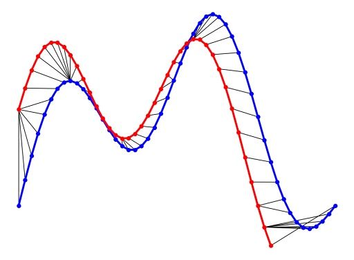
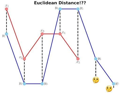
As you can see in the figure above, the DTW distance between the two signals is particularly powerful when the signals have similar patterns. The extrema, or the maximum and minimum points, between the two signals are correctly mapped. Unlike Euclidean distance, we may also see many-to-one mapping when DTW distance is used, particularly if the two signals have different lengths.
You may spot an issue with dynamic time warping from the figure above. Can you guess what it is?
The issue is that the head and tail of the time series don’t properly match. This is because the DTW algorithm can’t afford the warping invariance at the endpoints. The result is that a small difference at the sequence endpoints will tend to contribute disproportionately to the estimated similarity, according to a study on the effects of endpoints in time warping.
Dynamic Time Warping Advantages
DTW is an algorithm that can help you find an optimal alignment between two sequences and is a useful distance metric to have in your toolbox for several reasons:
- Non-linear sequences: DTW is useful when working with two non-linear sequences, particularly if one sequence is a non-linear stretched or shrunk version of the other. The warping path is a combination of chess king moves that starts from the head of two sequences and ends with their tails.
- Sequences of varying lengths: DTW works well with sequences that are different lengths, making it a valuable tool for handling time series models that aren’t aligned.
- Complex sequences: DTW can help align more complicated sequences that involve local shifts, such as measuring the different rates at which people talk.
- Noisy environments: Because DTW can align different time series models, it is able to perform well even in noisy data environments.
Frequently Asked Questions
What is dynamic time warping (DTW)?
Dynamic time warping (DTW) is a technique that makes it possible to compare two time series models that don’t sync up, minimizing the Euclidean distance between both models to align them as closely as possible.
How is DTW different from Euclidean distance?
Euclidean can be calculated only if two sequences are the same length. On the other hand, DTW can align sequences of different lengths, making it a better option for handling time series.
Where is DTW commonly used?
DTW is ideal for sequences that are of varying lengths, overly complex or non-linear, making it useful for applications like data mining, financial market analysis and speech recognition.