Regression models, both single and multivariate, are the backbone of many types of machine learning. Using the structure you specify, these tools create equations that match the modeled data set as closely as possible. Regression algorithms create the optimal equation by minimizing the error between the results predicted by the model and the provided data.
That said, no regression model will ever be perfect (and if your model does appear to be nearly perfect I recommend you check for overfitting). There will always be a difference between the values predicted by a regression model and the actual data. Those differences will change dramatically as you change the structure of the model, which is where residuals come into play.
How Do You Find Residuals?
The residual for a specific data point is the difference between the value predicted by the regression and the observed value for that data point. Calculating the residual provides a valuable clue into how well your model fits the data set. A poorly fit regression model will yield residuals for some data points that are very large, which indicates the model is not capturing a trend in the data set. A well-fit regression model will yield small residuals for all data points.
Let’s talk about how to calculate residuals.
Creating an Example Data Set
In order to calculate residuals we first need a data set for the example. We can create a fairly trivial data set using Python’s Pandas, NumPy and scikit-learn packages. You can use the following code to create a data set that’s essentially y = x with some noise added to each point.
import pandas as pd
import numpy as np

data = pd.DataFrame(index = range(0, 10))
data['Independent'] = data.index

np.random.seed(0)
bias = 0
stdev = 15

data['Noise'] = np.random.normal(bias, stdev, size = len(data.index))
data['Dependent'] = data['Independent'] * data['Noise']/100 + data['Independent']
That code performs the following steps:
- Imports the Pandas and NumPy packages you’ll need for the analysis
- Creates a Pandas data frame with 10
Independentvariables represented by the range between0and10 - Calculates a randomized percent error (
Noise) for each point using a normal distribution with a standard deviation of 15 percent - Calculates some
Dependentdata which is equal to theIndependentdata plus the error driven by theNoise
We can now use that data frame as our sample data set.
Implementing a Linear Model
The Dependent variable is our y data series, and the Independent variable is our x. Now we need a model which predicts y as a function of x. We can do that using scikit-learn’s linear regression model with the following code.
from sklearn.linear_model import LinearRegression

model = LinearRegression()
model.fit(np.array(data['Independent']).reshape((-1, 1)), data['Dependent'])
data['Calculated'] = model.predict(np.array(data['Independent']).reshape((-1, 1)))
That code works as follows:
- Imports the scikit-learn
LinearRegressionmodel for use in the analysis - Creates an instance of
LinearRegressionwhich will become our regression model - Fits the model using the
IndependentandDependentvariables in our data set - Adds a new column to our data frame storing the dependent values as predicted by our model (
Calculated)
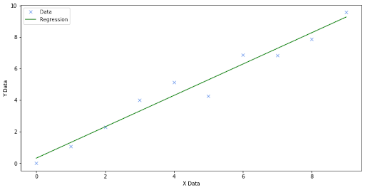
If the model perfectly matches the data set, then the values in the Calculated column will match the values in the Dependent column. We can plot the data to see if it does or not.
…nope.
Calculating the Model Residuals
We could have seen that coming because we used a first-order linear regression model to match a data set with known noise in it. In other words, we know that this model would have perfectly fit y = x, but the variation we added in each data point made every y a bit different from the corresponding x. Instead of perfection, we see gaps between the Regression line and the Data points. Those gaps are called the residuals. See the following plot which highlights the residual for the point at x = 4.

To calculate the residuals we need to find the difference between the calculated value for the independent variable and the observed value for the independent variable. In other words, we need to calculate the difference between the Calculated and Independent columns in our data frame. We can do so with the following code:
data['Residual'] = data['Calculated'] - data['Dependent']We can now plot the residuals to see how they vary across the data set. Here’s an example of a plotted output:
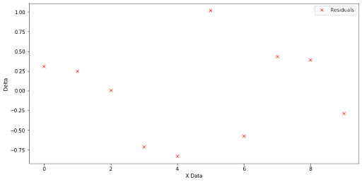
Notice how some of the residuals are greater than zero and others are less than zero. This will always be the case! Since linear regression reduces the total error between the data and the model to zero the result must contain some errors less than zero to balance out the errors that are greater than zero.
You can also see how some of the errors are larger than others. Several of the residuals are in the +0.25 – 0.5 range, while others have an absolute value in the range of 0.75 – 1. These are the signs that you look for to ensure a model is well fit to the data. If there’s a dramatic difference, such as a single point or a clustered group of points with a much larger residual, you know that your model has an issue. For example, if the residual at x = 4 was -5 that would be a clear sign of an issue. Note that a residual that large would probably indicate an outlier in the data set, and you should consider removing the point using interquartile range (IQR) methods.
Identifying a Poor Model Fit
To highlight the argument that residuals can demonstrate a poor model fit, let’s consider a second data set. To create the new data set I made two changes. The changed lines of code are as follows:
data = pd.DataFrame(index = range(0, 100))

data['Dependent'] = data['Independent'] * data['Noise']/100 + data['Independent']**2
The first change increased the length of the data frame index to 100. This created a data set with 100 points, instead of the prior 10. The second change made the Dependent variable be a function of the Independent variable squared, creating a parabolic data set. Performing the same linear regression as before (not a single letter of code changed) and plotting the data presents the following:
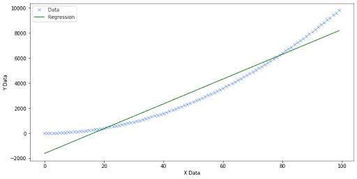
Since this is just an example meant to demonstrate the point, we can already tell that the regression doesn’t fit the data well. There’s an obvious curve to the data, but the regression is a single straight line. The regression under-predicts at the low and high ends, and over-predicts in the middle. We also know it’s going to be a poor fit because it’s a first-order linear regression on a parabolic data set.
That said, this visualization effectively demonstrates how examining the residuals can show a model with a poor fit. Consider the following plot, which I generated using the exact same code as the prior residuals plot.
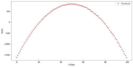
Can you see the trend in the residuals? The residuals are very negative when the X Data is both low and high, indicating that the model is under-predicting the data at those points. The residuals are also positive when the X Data is around the midpoint, indicating the model is over-predicting the data in that range. Clearly the model is the wrong shape and, since the residuals curve only shows one inflection point, we can reasonably guess that we need to increase the order of the model by one (to two).
If we repeat the process using a second-order regression, we obtain the following residuals plot.
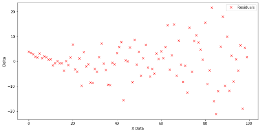
The only discernible pattern here is that the residuals increase as the X Data increases. Since the Dependent data includes noise, which is a function of the X Data, we expect that to happen. What we don’t see are very large residuals, or indications of a different shape to the data set. This means we now have a model that fits the data set well.
And with that, you’re all set to start evaluating the performance of your machine learning models by calculating and plotting residuals!
Frequently Asked Questions
What are residuals in regression analysis?
Residuals are the differences between the predicted values from a regression model and the actual observed values. They help measure how well a model fits the data.
Why are residuals important?
Residuals show whether a regression model is capturing the underlying trend in the data. Large residuals can signal poor model fit, noise or potential outliers.
How do you calculate residuals in Python?
Residuals can be calculated by subtracting the predicted dependent values from the observed dependent values, then storing the results in a new column.
What does a residual plot tell you?
A residual plot shows how errors vary across data points. Random scatter suggests a good fit, while visible patterns indicate model misspecification.


