Grouping Data With R: A Guide

Data by itself can be quite interesting, but even if you’re dealing with a small data set, the chances are that you’ll have to summarize or aggregate it. That’s where we’ll need groups.  

While it’s nice to know the total amount of sales, it’s often more useful to know the total amount of sales either by salesperson or by month.

Grouping data is undeniably essential for data analysis, and I’ll investigate some of the methods for doing so with R, Tidyverse and the dplyr package.

The data set I’ll use for the next examples comes from Kaggle and contains Spotify’s top songs from 2010 to 2019.

library("tidyverse")

df <- read_csv('data/spotify.csv') %>%
 rename(genre = `top genre`)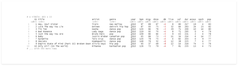

Now our data set is loaded to a Tibble, which contains 603 records and 15 columns.

How to Group Data With R

Now, let’s group the data by genre and see what we get.

# group by genre
df %>%
 group_by(genre)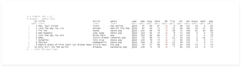

There’s almost no difference in the results, but now the second line has some information about the group. It may seem that nothing changed, but since the data is grouped, it’ll be treated differently in the next operations.

How to Analyze Data While Grouping in R

We can use summarise to observe this difference, first, let’s do it without groups.

df %>%
 summarise(summary = mean(bpm))

Since we didn’t have any groups, R returns the mean value for the whole data set.

df %>%
 group_by(genre) %>%
 summarise(mean_bpm = mean(bpm))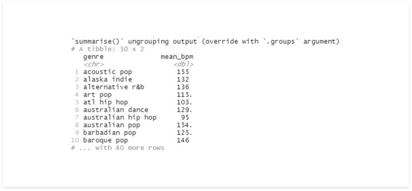

Now, we have unique values on the genre and their respective average beats per minute (bpm).

Note that this new Tibble doesn’t have the group’s information anymore.

How to Create a New Column While Grouping in R 

Now we’ll create a new column with mutate, instead of summarise. First, we’ll see the result without grouping:

# mutate without grouping
df %>%
 mutate(mean_bpm = (bpm - mean(bpm))^2) %>%
 select(genre, mean_bpm)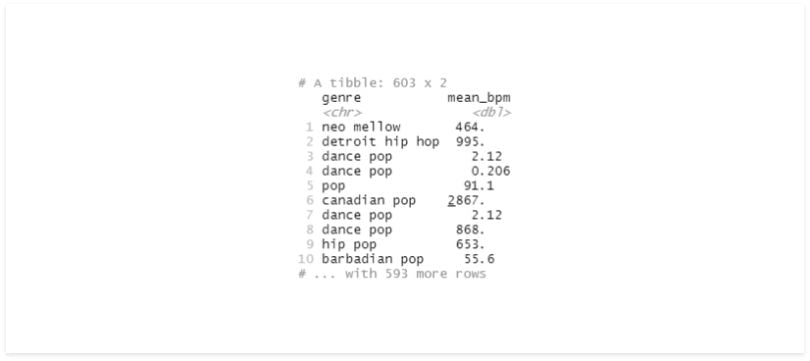

# mutate with grouping
df %>%
 group_by(genre) %>%
 mutate(mean_bpm = (bpm - mean(bpm))^2) %>%
 select(genre, mean_bpm)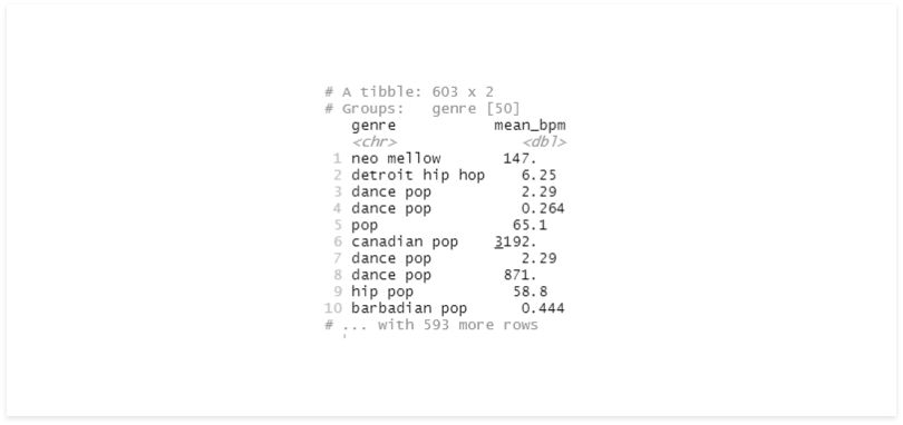

The results are very different. On the first one, we iterated each record, getting its bpm, then divided it by the mean of all records and squared the result.

On the second, we did the same thing but divided by the mean bpm of the records in that group. We can also see that even after using mutate, our data is still grouped.

How to Ungroup Your Data in R

If we need to change that, we can easily do so with ungroup() to perform other operations.

df %>%
 group_by(genre) %>%
 mutate(mean_bpm = mean(bpm) %>%
 select(genre, mean_bpm) %>%
 mutate(my_grouped_sum = sum(mean_bpm)) %>%
 ungroup() %>%
 mutate(my_regular_sum = sum(mean_bpm))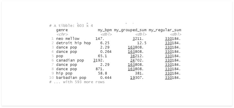

It’s easy to mistake your data set with its grouped version, so it’s  recommended that you always ungroup your data before saving the results to a variable.

We know that group_by will return a Tibble very similar to our standard Tibble. The difference is in how it’ll handle the next operations.

RelatedThe Ultimate Guide to Relational Operators in R

How to Group Multiple Fields in R

Using multiple fields to group the data is also quite easy; we can add them as parameters on our group_by.

# multiple fields
df %>%
 group_by(genre, year) %>%
 summarise(rec_count = n()) %>%
 arrange(desc(year), desc(rec_count))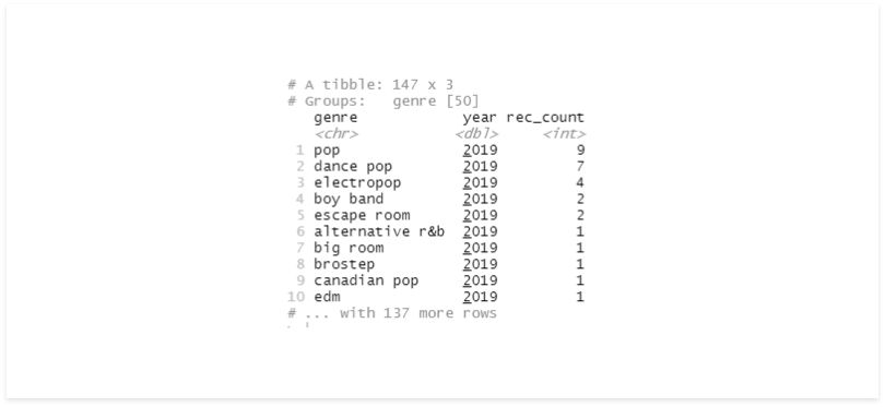

The last time we used summarise, it returned a Tibble without groups. Now that we’re using multiple variables, we still have a group in the result.

While the grouped and ungrouped Tibble look similar, they are not. Let’s repeat this code, adding a column with the count after summarise and another after ungrouping.

# multiple fields
df %>%
 group_by(genre, year) %>%
 summarise(genre_year_count = n()) %>%
 arrange(desc(year), desc(genre_year_count)) %>%
 mutate(genre_count = n()) %>%
 ungroup() %>%
 mutate(total_count = n())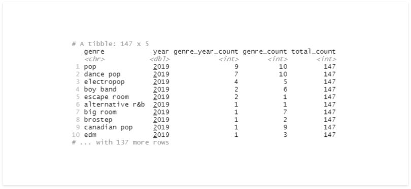

Sometimes we might perform some operations with a group and then need to add another field to our group_by.

Using a group_by after the other replaces the previous, but we can set the parameter add to “true” to complete that action.

df %>%
 group_by(genre) %>%
 mutate(mean_bpm_genre = mean(bpm)) %>%
 group_by(year, add = TRUE) %>%
 mutate(mean_bpm_genre_year = mean(bpm)) %>%
 select(genre, year, mean_bpm_genre, mean_bpm_genre_year)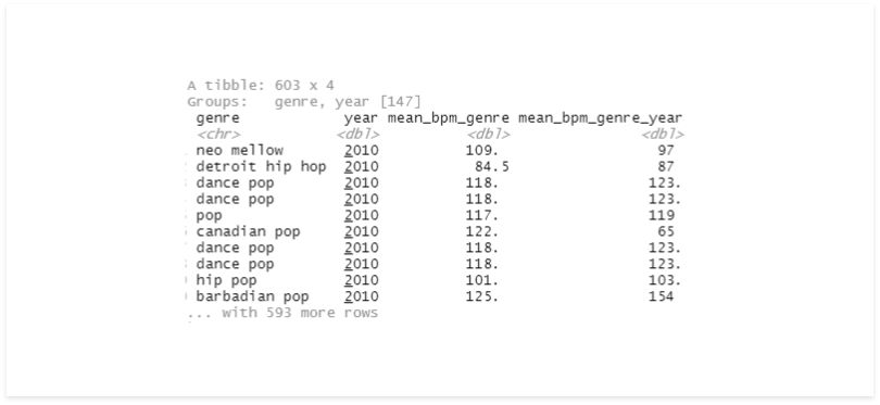

Group in R With Variables and Functions

Now, let’s try using group_by more programmatically. We’ll try to define a function, pass the group as a parameter, perform a simple count and get the results.

my_func <- function(df, group){
 df %>%
   group_by(group) %>%
   summarise(my_count = n()) %>%
   arrange(desc(my_count))
}

my_func(df, 'year')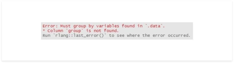

It isn’t so simple. We need to make a few adjustments to make this work. One possible solution is to use quosure.

my_func <- function(df, group){
 df %>%
   group_by(!!group) %>%
   summarise(my_count = n()) %>%
   arrange(desc(my_count))
}

my_group = quo(year)
my_func(df, my_group)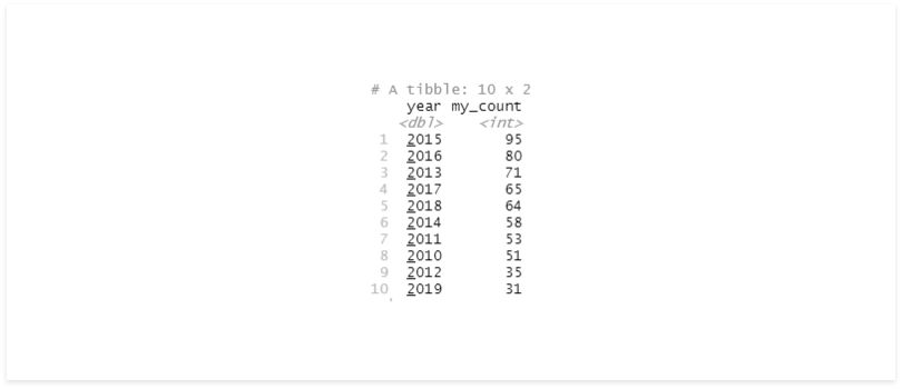

We could also use group_by_.

Many dplyr verbs have an alternative version with an extra underline at the end. Those can help us use methods such as group_by more programmatically.  

Dplyr uses non-standard evaluation for most of its single table verbs, including: filter(), mutate(), summarise(), arrange(), select() and group_by(). While it’s faster to type and makes it possible to translate the code into SQL, it’s difficult to program.

Let’s try the function again, this time with group_by_.

my_func <- function(df, group){
 df %>%
   group_by_(group) %>%
   summarise(my_count = n()) %>%
   arrange(desc(my_count))
}

my_func(df, 'genre')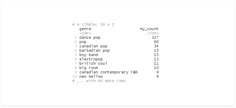

That’s easier than using quosure, it’s more readable and it yields the same result.

We explored the basics of group_by, how to use multiple fields to group our data, the differences between a grouped and a regular Tibble, and how to use group_by_ to achieve more programmatic solutions.

RelatedThe Ultimate Guide to Logical Operators in R

Grouping in R Variants

There are some variants such as group_by_all and group_by_if. As much as they’re considered to be superseded by the use of across, it’s worth getting a look at them too.

Group_by_all

The name gives it away, group_by_all uses every field in the data set. As mentioned, the same can be done using group_by and across.

new_df <- select(df, genre, year)

new_df %>%
 group_by_all() %>%
 summarise(my_cnt = n()) %>%
 arrange(desc(my_cnt))

new_df %>%
 group_by(across()) %>%
 summarise(my_cnt = n()) %>%
 arrange(desc(my_cnt))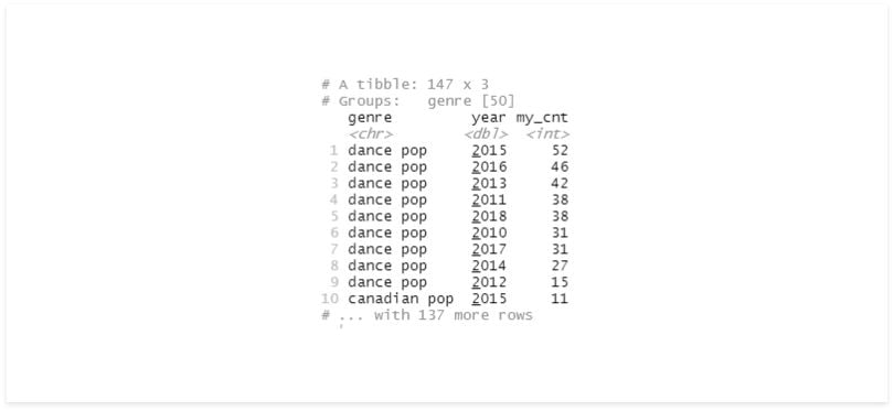

I’ve never found myself in a situation where I needed to group all columns, but it could come in handy in some cases, and it’s good to know it exists.

Group_by_if

Another fascinating variant is group_by_if, which allows us to use a function to select the fields.

# group_by_if
new_df <- df %>%
 mutate(artist = as.factor(artist),
        genre = as.factor(genre))

new_df %>%
 group_by_if(is.factor) %>%
 summarise(my_cnt = n()) %>%
 arrange(desc(my_cnt))

new_df %>%
 group_by(across(where(is.factor))) %>%
 summarise(my_cnt = n()) %>%
 arrange(desc(my_cnt))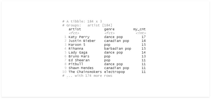

Let’s try another example with a custom function. We’ll group the columns where any record contains the word “dance” on them.

new_df %>%
 group_by_if(function(x) any(grepl("dance", x, fixed=TRUE))) %>%
 summarise(my_cnt = n())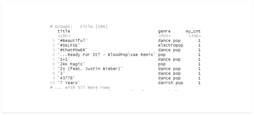

Group_split

Sometimes we’ll also need different treatments for different groups. That is made simple with group_split, which separates our data into a list of Tibbles, one for each group.

In this example, we’ll group the data by year, split, and save the result to a variable called df_list.

To test, we can select an index of this list. In return, we should get a Tibble containing only the records of one year.

# split
df_list <- df %>%
 group_by(year) %>%
 group_split()

df_list[[10]]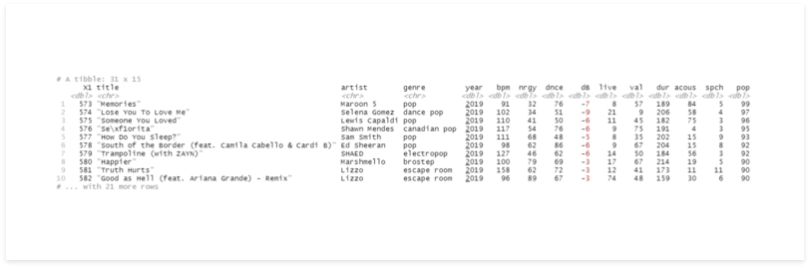

Group_nest

A more sophisticated solution for separating our groups is group_nest, which returns a Tibble containing the grouped columns and the data from those respective groups.

# nest
df_nest <- df %>%
 group_nest(genre, year)

df_nest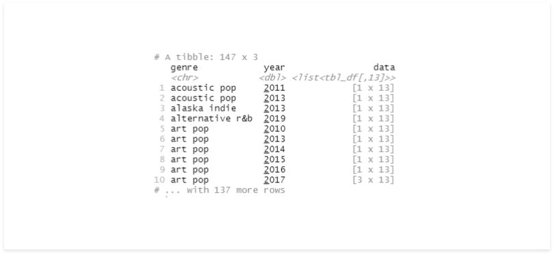

There are plenty of ways to group our data and manipulate it once it’s grouped, but I believe we covered enough for the basics.

Frequently Asked Questions