Pipe in R: A Guide

Pipe in R, written as |>, is a native feature of the R language since version 4.1.0. It takes the output of one function and passes it into another function as an argument. Pipe is R’s most important operator for data processing.

Data analysis often involves many steps. A typical journey from raw data to results might involve filtering cases, transforming values, summarizing data and then running a statistical test. Pipe in R links all these steps together, while keeping our code efficient and readable.

What Does Pipe in R Do?

The pipe operator, formerly written as %>%, was a longstanding feature of the magrittr package for R. The new version, written as |>, is largely the same. It takes the output of one function and passes it into another function as an argument. This allows us to link a sequence of analysis steps.

To visualize this process, imagine a factory with different machines placed along a conveyor belt. Each machine is a function that performs a stage of our analysis, like filtering or transforming data. The pipe works like a conveyor belt, transporting the output of one machine to another for further processing.

More on RGuide to Logical Operators in R (OR, NOT and AND in R)

How to Use Pipe in R With an Example

We can see exactly how this works in a real example using the mtcars data set. This data set comes with base R and contains data about the specs and fuel efficiency of various cars.

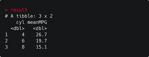
The code below groups the data by the number of cylinders in each car, and then returns the mean miles-per-gallon of each group. Make sure to install the dplyr package before running this code, since it includes the group_by and summarise functions.

library(dplyr)
result <- mtcars |>
   group_by(cyl) |>
   summarise(meanMPG = mean(mpg))

The pipe operator feeds the mtcars dataframe into the group_by function, and then the output of group_by into summarise. The outcome of this process is stored in the tibble result, shown below.

Although this example is very simple, it demonstrates the basic pipe workflow. To go even further, I’d encourage playing around with this. Perhaps swap and add new functions to the ‘pipeline’ to gain more insight into the data. Doing this is the best way to understand how to work with the pipe.

Additional Pipes in R to Know

Before R version 4.1.0 introduced the native pipe, the go-to pipe operator in R was part of the magrittr package. The magrittr pipe, written as %>%, has much of the same functionality as the native pipe. The two are largely interchangeable, and the magrittr pipe is only preferred for its flexibility in a small set of cases. Despite this, there are three other pipes in the magrittr package that are worth knowing for their extra functionality.

The Assignment Pipe

The assignment pipe, written %<>%, is shorthand for assigning the outcome of a pipe sequence to a variable at the start of a pipe sequence. As an example, we can use this to store the sum of the numbers in a vector, sum_data, to a variable with the same name. While this creates repetition using a traditional pipe, an assignment pipe can make this look cleaner.

# Native pipe example
sum_data <- 1:5
sum_data <- sum_data |>
    sum()
# Assignment pipe example (gives the same output)
library(magrittr)
sum_data <- 1:5
sum_data %<>%
    sum()

The Tee Pipe

Sometimes, we may want to insert a function that doesn’t return an output for further processing into a pipe sequence. The tee pipe, written %T>%, pipes data to the next two functions in the pipe sequence, allowing the first to return a result without affecting the rest of the sequence.

mtcars %>%
    select(mpg, wt) %T>%
    plot() %>%
    summarise(meanMPG = mean(mpg))

To see this in action, we can set up a pipe sequence to plot variables from the mtcars data set and calculate an average of a column. The tee pipe in this sequence passes on the data from the select function to plot, producing a scatterplot of that data. The tee pipe also passes the output from select on to summarise, letting the pipe sequence continue. If we used a native pipe here, the plot wouldn’t output any data for summarise to process in the next step of the chain, which would cause an error.

Output:
  meanMPG
1 20.09062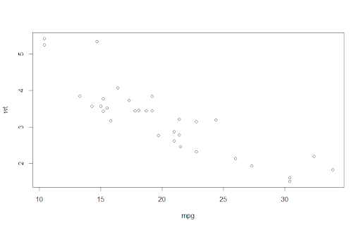

The Exposition Pipe

The exposition pipe, written %$%, exposes names from data sets being passed through the pipe to the next function. To see this in use, we can create a simple bar plot of the results of our first example. Using the exposition pipe, we can refer to the column names of the result dataframe inside the barplot function, allowing us to create the plot concisely. 

result %$%
    barplot(meanMPG, names.arg = cyl)

Output:

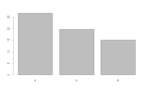
If we didn’t use the exposition pipe, we’d have to pull the meanMPG and cyl columns from our data set separately and give them to barplot, which is less efficient.

Why Use Pipe in R?

The pipe operator has a huge advantage over any other method of processing data in R: It makes processes easy to read. If we read |> as “then”, the code from the previous section is very easy to digest as a set of instructions in plain English:

Load dplyr package
To get our result, take the mtcars dataframe, THEN
   Group its entries by number of cylinders, THEN
   Compute the mean miles-per-gallon of each group

This is far more readable than if we were to express this process in another way. The two options below are different ways of expressing the previous code, but both are worse for a few reasons.

# Option 1: Store each step in the process sequentially
result <- group_by(mtcars, cyl)
result <- summarise(result, meanMPG = mean(mpg))

# Option 2: chain the functions together
> result <- summarise(
               group_by(mtcars, cyl),
               meanMPG = mean(mpg))

“Option 1” gets the job done, but overwriting our output dataframe result in every line is problematic. For one, doing this for a procedure with lots of steps isn’t efficient and creates unnecessary repetition in the code. This repetition also makes it harder to identify exactly what is changing on each line in some cases.

“Option 2” is even less practical. Nesting each function we want to use gets ugly fast, especially for long procedures. It’s hard to read and harder to debug. This approach also makes it tough to see the order of steps in the analysis, which is bad news if you want to add new functionality later.

Also, if you’re fed up with awkwardly typing |>, The slightly easier keyboard shortcut CTRL + SHIFT + M will print a pipe in RStudio!

It’s easy to see how using the pipe can substantially improve most R scripts. It makes analyses more readable, removes repetition, and simplifies the process of adding and modifying code. Is there anything it can’t do?

More on RHow to Use strsplit() Function in R

What Are the Limitations of Pipe in R?

Although it’s immensely handy, the pipe isn’t useful in every situation. Here are a few of its limitations:

• Because it chains functions in a linear order, the pipe is less applicable to problems that include multidirectional relationships.
• The pipe can only transport one object at a time, meaning it’s not so suited to functions that need multiple inputs or produce multiple outputs.
• It doesn’t work with functions that use the current environment, nor functions that use lazy evaluation. 

These things are to be expected. Just as you’d struggle to build a house with a single tool, no lone feature will solve all your programming problems. But for what it’s worth, the pipe is still pretty versatile. Although this piece focused on the basics, there’s plenty of scope for using the pipe in advanced or creative ways. I’ve used it in a variety of scripts, data-focused and not, and it’s made my life easier in each instance.

Pipes are great. They turn your code into a list of readable instructions and have lots of other practical benefits. So now you know about pipes, use them, and watch your code turn into a narrative.

Frequently Asked Questions