Double deep Q-learning is a reinforcement learning algorithm and variation of the deep Q-learning algorithm used to reduce the overestimation of action values calculated in deep Q-learning. It does this by decomposing the max operation in the target value into separate action selection and action evaluation processes.
What Is Double Deep Q-Learning?
Double deep Q-learning is a variation of the deep Q-learning reinforcement algorithm that aims reduce the overestimation of action values calculated in deep Q-learning, and does so by decomposing the max operation in the target value into action selection and action evaluation processes.
In the last installment in this series on self-learning AI agents, I introduced deep Q-Learning as an algorithm that can be used to teach AI to behave and solve tasks in discrete action spaces. However, this approach is not without its shortcomings that can potentially result in lower performance of the AI agent.
In what follows, I’ll introduce how deep Q-learning can be extended to what we call double deep Q-learning, which generally leads to better AI agent performance.
But first, let’s go over some basics about reinforcement learning and standard deep Q-learning before explaining double deep Q-learning.
First, What Is the Action-Value Function?
In the first and second part of this series, I introduced the action-value function Q(s,a) as the expected return G_t the AI agent would get by starting in state s, taking action a and then following a certain policy π.
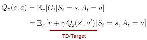
Q(s,a)The right part of the equation is also called the temporal difference target (TD-Target). The TD-Target is the sum of the immediate reward r the agent received for the action a in state s and the discounted value Q(s’,a’) (a’ being the action the agent will take in the next state s’).
Q(s,a) tells the agent the value (or quality) of a possible action a in a particular state s.
Given a state s, the action-value function calculates the quality/value for each possible action a_i in this state as a scalar value. Higher quality means a better action with regards to the given objective. For an AI agent, a possible objective could be learning how to walk or how to play chess against humans.
Following a greedy policy w.r.t Q(s,a) — i.e. taking the actions a’ that result in the highest values of Q(s,a’) — leads to the Bellman optimality equation, which gives a recursive definition for Q(s,a). We can also use the Bellman equation to recursively calculate all values Q(s,a) for any given action or state.
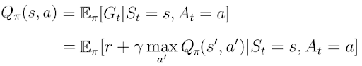
In part two of this series, I introduced temporal difference learning as a better approach to estimate the values Q(s,a). The objective in temporal difference learning was to minimize the distance between the TD-Target and Q(s,a), which suggests a convergence of Q(s,a) towards its true values in the given environment. This is Q-learning.
What Is Deep Q-Learning and Deep Q-Networks?
We’ve seen that a neural network approach turns out to be a better way to estimate Q(s,a). Nevertheless, the main objective stays the same: the minimization of the distance between Q(s, a) and TD-Target (or temporal distance of Q(s,a)). We can express this objective as the minimization of the error loss function:
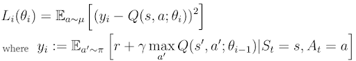
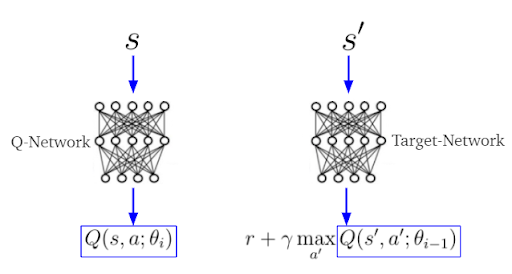
In deep Q-learning, we estimate TD-target y_i and Q(s,a) separately by two different neural networks, often called the target- and Q-networks (figure 4). The parameters θ(i-1) (weights, biases) belong to the target-network, while θ(i) belong to the Q-network.
The actions of the AI agents are selected according to the behavior policy µ(a|s). On the other side, the greedy target policy π(a|s) selects only actions a’ that maximize Q(s, a) (used to calculate the TD-target).
s being the current and s’ the next stateWe can accomplish minimization of the error loss function by usual gradient descent algorithms we use in deep learning.
The Problem With Deep Q-Learning
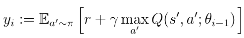
Deep Q-learning is known to sometimes learn unrealistically high action values because it includes a maximization step over estimated action values, which tends to prefer overestimated to underestimated values. We can see this in the TD-target y_i calculation.
It’s still more or less an open question whether overestimations negatively affect performances of AI agents in practice. Over-optimistic value estimates are not necessarily a problem in and of themselves. If all values would be uniformly higher, then the relative action preferences are preserved and we would not expect the resulting policy to be any worse.
If, however, the overestimations are not uniform and not concentrated at states about which we wish to learn more, then they might negatively affect the quality of the resulting policy.
How Does Double Deep Q-Learning Work?
The idea of double Q-learning is to reduce overestimations by decomposing the max operation in the target into action selection and action evaluation.
In the vanilla implementation, the action selection and action evaluation are coupled. We use the target-network to select the action and estimate the quality of the action at the same time. What does this mean?
The target-network calculates Q(s, a_i) for each possible action a_i in state s. The greedy policy decides upon the highest values Q(s, a_i) which selects action a_i. This means the target-network selects the action a_i and simultaneously evaluates its quality by calculating Q(s, a_i). Double Q-learning tries to decouple these procedures from one another.
In double Q-learning the TD-target looks like this:
As you can see, the max operation in the target is gone. While the target-network with parameters θ(i-1) evaluates the quality of the action, the Q-network determines the action that has parameters θ(i). This procedure is in contrast to the vanilla implementation of deep Q-learning where the target-network was responsible for action selection and evaluation.
We can summarize the calculation of new TD-target y_i in the following steps:
-
Q-network uses next state
s’to calculate qualitiesQ(s’,a)for each possible actionain states’ -
Argmax operation applied on
Q(s’,a)chooses the actiona*that belongs to the highest quality (action selection). -
The quality
Q(s’,a*)(determined by the target-network) that belongs to the actiona*(determined by the Q-network) is selected for the calculation of the target (action evaluation).
We can visualize the process of double Q-learning like this:
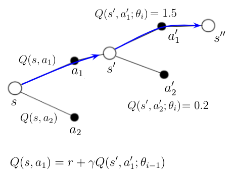
An AI agent is at the start in state s. He knows, based on some previous calculations, the qualities Q(s, a_1) and Q(s, a_2) for two possible actions in that state. The agent decides to take action a_1 and ends up in state s’.
The Q-network calculates the qualities Q(s’, a_1’) and Q(s, a_2’) for possible actions in this new state. Action a_1’ is picked because it results in the highest quality according to the Q-network.
We can now calculate the new action-value Q(s, a1) for action a_1 in state s with the equation in the figure 2, where Q(s’,a_1’) is the evaluation of a_1’ is determined by the target-network.
Double Deep Q-Learning Example
This example of OpenAI’s Gym CartPole problem was solved with the double Q-learning algorithm, presented here — as well as some techniques from last time. The well-documented source code can be found in my GitHub repository.
run_training.py to start the algorithm.
Double Deep Q-Learning vs. Deep Q-Learning
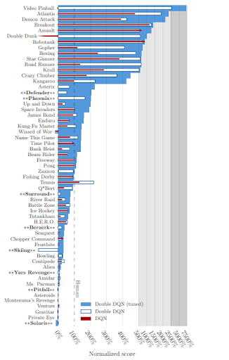
In this 2015 study, researchers tested deep Q-networks (DQNs) and double deep Q-networks (double DQNs) on several Atari 2600 games. You can see the normalized scores achieved by AI agents of those two methods, as well as the comparable human performance, in figure 3.
You can clearly see that these two versions of double DQNs achieve better performances in this area than the vanilla deep Q-learning algorithm implementation.
With deep Q-Learning and deep (double) Q-learning we learned to control an AI in discrete action spaces, where the possible actions may be as simple as going left or right, up or down.
However, many real-world applications of reinforcement learning, such as the training of robots or self-driving cars, require an agent to select optimal actions from continuous spaces where there are (theoretically) an infinite amount of possible actions. This is where stochastic policy gradients come into play, the topic of the next article of this series.
Frequently Asked Questions
What is double deep Q-learning?
Double deep Q-learning variation of the deep Q-learning reinforcement learning algorithm used to reduce the overestimation of action values in deep Q-learning. It performs this reduction by decomposing the max operation in the target value into separate action selection and action evaluation processes.
Is double Q-learning better than Q-learning?
Double deep Q-learning is generally considered to improve the performance and stability of an AI agent in comparison to standard Q-learning. This is due to double deep Q-learning reducing the overestimation of action values in calculations, as Q-learning tends to prefer overestimated action values.