Sorting is the process of organizing elements in a structured manner. Quicksort is one of the most popular sorting algorithms that uses nlogn comparisons to sort an array of n elements in a typical situation. Quicksort is based on the divide-and-conquer strategy.
QuickSort Explained
Quicksort is a sorting algorithm that uses a divide-and-conquer strategy to sort an array. It does so by selecting a pivot element and then sorting values larger than it on one side and smaller to the other side, and then it repeats those steps until the array is sorted. It is useful for sorting big data sets.
We’ll take a look at the Quicksort algorithm in this tutorial and see how it works.
What Is Quicksort?
Quicksort is a fast sorting algorithm that works by splitting a large array of data into smaller sub-arrays. This implies that each iteration splits the input into two components, sorts them and then recombines them. The technique is highly efficient for big data sets because its average and best-case complexity is O(n*logn).
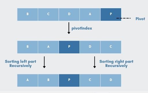
There might be a few drawbacks to Quicksort, but it performs well in practice and can outperform other sorting algorithms in speed and space efficiency. Quicksort was created by Tony Hoare in 1961 and remains one of the fastest, most effective general-purpose sorting algorithms available today.
How Does Quicksort Work?
Quicksort works by recursively sorting the sub-lists to either side of a given pivot and dynamically shifting elements inside the list around that pivot.
As a result, the Quicksort method can be summarized in three steps:
- Pick: Select an element.
- Divide: Split the problem set, move smaller parts to the left of the pivot and larger items to the right.
- Repeat and combine: Repeat the steps and combine the arrays that have previously been sorted.
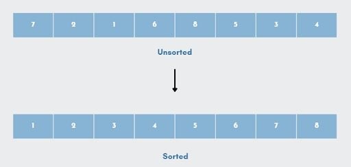
Let’s take a look at an example to get a better understanding of the Quicksort algorithm. In this example, the array below contains unsorted values, which we will sort using Quicksort.
1. Select a Pivot
The process starts by selecting one element known as the pivot from the list. This can be any element. A pivot can be:
- Any element at random.
- The first or last element.
- Middle element.
For this example, we’ll use the last element, 4, as our pivot.
2. Rearrange the Array
Now, the goal here is to rearrange the list such that all the elements less than the pivot are to its left, and all the elements greater than the pivot are to the right of it. Remember:
- The pivot element is compared to all of the items starting with the first index. If the element is greater than the pivot element, a second pointer is appended.
- When compared to other elements, if a smaller element than the pivot element is found, the smaller element is swapped with the larger element identified before.
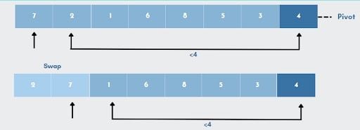
Let’s simplify the above example:
- Every element, starting with
7, will be compared to the pivot(4). A second pointer will be placed at7because7is bigger than4. - The next element, element
2will now be compared to the pivot. As2is less than4, it will be replaced by the bigger figure7which was found earlier. - The numbers
7and2are swapped. Now, pivot will be compared to the next element,1which is smaller than4. - So once again,
7will be swapped with1. - The procedure continues until the next-to-last element is reached, and at the end, the pivot element is then replaced with the second pointer. Here, number
4(pivot) will be replaced with number6.
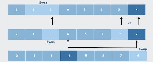
As elements 2, 1, and 3 are less than 4, they are on the pivot’s left side. Elements can be in any order: ‘1’,’2’,’3’, or ‘3’,’1’,’2’, or ‘2’,’3’,’1’. The only requirement is that all of the elements must be less than the pivot. Similarly, on the right side, regardless of their sequence, all components should be greater than the pivot.
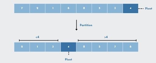
In other words, the algorithm searches for every value that is smaller than the pivot. Values smaller than pivot will be placed on the left, while values larger than pivot will be placed on the right. Once the values are rearranged, it will set the pivot in its sorted position.
3. Divide the Subarrays
Once we have partitioned the array, we can break this problem into two sub-problems. First, sort the segment of the array to the left of the pivot, and then sort the segment of the array to the right of the pivot.
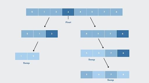
- In the same way that we rearranged elements in step two, we’ll pick a pivot element for each of the left and right sub-parts individually.
- Now, we’ll rearrange the sub-list such that all the elements are less than the pivot point, which is toward the left. For example, element
3is the largest among the three elements, which satisfies the condition. Hence, the element,3, is in its sorted position. - In a similar manner, we will again work on the sub-list and sort the elements
2and1. We will stop the process when we get a single element at the end. - Repeat the same process for the right-side sub-list. The subarrays are subdivided until each subarray consists of only one element.
- Now, the array is sorted.
Quicksort Advantages and Disadvantages
Advantages of Quicksort
Let’s cover a few key advantages of using Quicksort:
- It works rapidly and effectively.
- It has the best time complexity when compared to other sorting algorithms.
- QuickSort has a space complexity of
O(log n), making it an excellent choice for situations when space is limited.
Disadvantages of Quicksort
Despite being the fastest algorithm, Quicksort has a few drawbacks. Let’s look at some of the drawbacks of quicksort.
- This sorting technique is considered unstable since it doesn’t maintain the key-value pairs initial order.
- It isn’t as effective when the pivot element is the largest or smallest, or when all of the components have the same size. The performance of the quicksort is significantly impacted by these worst-case scenarios.
- It’s difficult to implement since it’s a recursive process, especially if recursion isn’t available.
Quicksort Algorithm Code Example
Quicksort Function Algorithm
//start –> Starting index,  end --> Ending index
Quicksort(array, start, end)
{
   if (start < end)
   {
      pIndex = Partition(A, start, end)
      Quicksort(A,start,pIndex-1)
      Quicksort(A,pIndex+1, end)
   }
}
Quicksort Partition Function Algorithm
The subarrays are rearranged in a certain order using the partition method. You will find various ways to partition. Here, we will see one of the most used methods.
partition (array, start, end)
{
    // Setting rightmost Index as pivot
    pivot = arr[end];

    i = (start - 1)  // Index of smaller element and indicates the
                   // right position of pivot found so far
for (j = start; j <= end- 1; j++)
    {
        // If current element is smaller than the pivot
        if (arr[j] < pivot)
        {
            i++;    // increment index of smaller element
            swap arr[i] and arr[j]
        }
    }
    swap arr[i + 1] and arr[end])
    return (i + 1)
}
How to Implement Quicksort in JavaScript
Let’s look at Quicksort programs written in JavaScript and Python programming languages. We’ll start by creating a function that allows you to swap two components.
function swap(arr, i, j)
{    let temp = arr[i];
    arr[i] = arr[j];
    arr[j] = temp;
}
Now, let’s add a function that uses the final element (last value) as the pivot, moves all smaller items to the left of pivot, and all larger elements to the right of the pivot, and places the pivot in the appropriate location in the sorted array.
function partition(arr, start, end) {

    // pivot
    let pivot = arr[end];

/* Index of a smaller element that specifies the pivot's correct position so far. */

 let i = (start - 1);

    for (let j = start; j <= end - 1; j++) {

        // If current element is smaller than the pivot
        if (arr[j] < pivot) {


            i++;
            swap(arr, i, j);
        }
    }
    swap(arr, i + 1, end);
    return (i + 1);
}
Next, let’s add the main function that will partition and sort the elements.
function quickSort(arr, start, end) {
    if (start < end) {

        // The partitioning index is represented by pi.

        let pi = partition(arr, start, end);

        // Separately sort elements before and after partition
        quickSort(arr, start, pi - 1);
        quickSort(arr, pi + 1, end);
    }
}
Let’s finish off by adding a function to print the array.
function printArray(arr, size) {
    for (let i = 0; i < size; i++)
        document.write(arr[i] + " ");

    document.write("");
}

// Let's start by sorting the unsorted.

let arr = [7, 2, 1, 6, 8, 5, 3, 4];
let n = arr.length;

document.write("Orginal array:" + arr);
quickSort(arr, 0, n - 1);
document.write("Sorted array:"+arr);
Here is the full code of Quicksort implementation for JavaScript:
// This function allows you to swap two components.
function swap(arr, i, j) {
    let temp = arr[i];
    arr[i] = arr[j];
    arr[j] = temp;
}

/* This function uses the last element as the pivot, and moves all smaller items to the left of pivot and all larger elements to the right of pivot, and
inserts pivot in the appropriate location in the sorted array. */

function partition(arr, start, end) {

    // pivot
    let pivot = arr[end];

/* Index of a smaller element that specifies the pivot's correct position so far. */

 let i = (start - 1);

    for (let j = start; j <= end - 1; j++) {

        // If current element is smaller than the pivot
        if (arr[j] < pivot) {


            i++;
            swap(arr, i, j);
        }
    }
    swap(arr, i + 1, end);
    return (i + 1);
}

/* The main function that implements QuickSort
          arr[] --> Array to be sorted,
          start --> Starting index,
          end --> Ending index
 */
function quickSort(arr, start, end) {
    if (start < end) {

        // The partitioning index is represented by pi.

        let pi = partition(arr, start, end);

        // Separately sort elements before
        // partition and after partition
        quickSort(arr, start, pi - 1);
        quickSort(arr, pi + 1, end);
    }
}

// Array printing function
function printArray(arr, size) {
    for (let i = 0; i < size; i++)
        document.write(arr[i] + " ");

    document.write("");
}

// Let's start by sorting the unsorted.

let arr = [7, 2, 1, 6, 8, 5, 3, 4];
let n = arr.length;

document.write("Orginal array:" + arr);
quickSort(arr, 0, n - 1);
document.write("Sorted array:"+arr);

How to Implement Quicksort in Python
Now, let’s look at Quicksort programs written in Python. We’ll start by creating a function which is responsible for sorting the first and last elements of an array.
def find_pviot_index(A,start,end):
    pivot=A[end]
    p_index=start
    for iter in range(start,end):
        if A[iter] <= pivot:
            A[p_index],A[iter]=A[iter],A[p_index]
            p_index+=1
    A[p_index],A[end]=pivot,A[p_index]
    return p_index
Next, we’ll add the main function that implements quick_sort.
def quick_sort(A,start,end):
    if start < end:
        pivot_index=find_pviot_index(A,start,end)
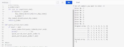
        print("--------------",A)
        quick_sort(A,start,pivot_index-1)
        quick_sort(A,pivot_index+1,end)
Let’s finish off by adding a function to print the array.
A=list()
n=int(input("Set of numbers you want to enter: "))
for x in range(0,n):
    num=int(input("Enter Num:"))
    A.append(num)
print("Orignal array:",A)
quick_sort(A,0,n-1)
print("Sorted array :",A)
Here is the full code of Quicksort implementation in Python.
#sorting the first and last elements of an array.
def find_pviot_index(A,start,end):
    pivot=A[end]
    p_index=start
    for iter in range(start,end):
        if A[iter] <= pivot:
            A[p_index],A[iter]=A[iter],A[p_index]
            p_index+=1
    A[p_index],A[end]=pivot,A[p_index]
    return p_index

#main sorting function
def quick_sort(A,start,end):
    if start < end:
        pivot_index=find_pviot_index(A,start,end)
        print("--------------",A)
        quick_sort(A,start,pivot_index-1)
        quick_sort(A,pivot_index+1,end)


#Driver code
A=list()
n=int(input("Set of numbers you want to enter: "))
for x in range(0,n):
    num=int(input("Enter Num:"))
    A.append(num)
print("Orignal array:",A)
quick_sort(A,0,n-1)
print("Sorted array :",A)
Time Complexity for Quicksort
Let’s look at the space and time complexity of Quicksort in the best, average and worst case scenarios. In general, the time consumed by Quicksort can be written as follows:
T(n) = T(k) + T(n-k-1) + O(n)Here, T(k) and T(n-k-1) refer to two recursive calls, while the last term O(n) refers to the partitioning process. The number of items less than pivot is denoted by k.
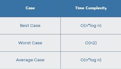
Quicksort Time Complexity
- Best-Case Time Complexity:
O (n*logn) - Average-Case Time Complexity:
O (n*logn) - Worst-Case Time Complexity:
O (n2)
1. Quicksort Best-Case Time Complexity
When the partitioning algorithm always chooses the middle element or near the middle element as the pivot, the best case scenario happens. Quicksort’s best-case time complexity is O (n*logn). The following is the best-case recurrence.
T(n) = 2T(n/2) + O(n)
//solution O(nLogn)
2. Quicksort Average-Case Time Complexity
This occurs when the array elements are in a disordered sequence that isn’t increasing or decreasing properly. QuickSort’s average case time complexity is O(n*logn). The following is the average-case recurrence.
T(n) = T(n/9) + T(9n/10) + O(n)
//solution O(nLogn)
3. Quicksort Worst-Case Time Complexity
The worst-case situation is when the partitioning algorithm picks the largest or smallest element as the pivot element every time. The worst-case time complexity of Quicksort is O (n2). The following is the worst-case recurrence.
T(n) = T(0) + T(n-1) + O(n)
//solution O(n2)
Quicksort Space Complexity
The space complexity for Quicksort is O(log n).

Quicksort Applications
The sorting algorithm is used to find information, and since Quicksort is the fastest, it is frequently used as a more efficient search approach.
- It’s applied wherever a stable sort isn’t required.
- Since it is tail-recursive, every call optimization can be done.
- It is useful in event-driven simulation and operational research.
Is Quicksort Better Than Other Sorting Algorithms?
Quicksort may have a few drawbacks, but it is the fastest and most efficient sorting algorithm available. Quicksort has an O(log n) space complexity, making it an excellent choice for situations where space is restricted.
Although the worst-case running time is always the same, Quicksort is often faster than HeapSort (nlogn). Quicksort takes up less space than heap sort due to the fact that a heap is nearly a full binary tree with pointers overhead. So, when it comes to sorting arrays, Quicksort is preferred.
Frequently Asked Questions
Is QuickSort still used?
Quicksort is a commonly used sorting algorithm for big data sorting, database management, graphics rendering, event-driven simulation and operational research.
What is the fastest sorting algorithm?
Quicksort is considered to be one of the fastest sorting algorithms, especially when applied to large data sequences.
Why is quicksort so efficient?
Quicksort’s efficiency is due to having a time complexity of O(nlogn) in best-case and average-case scenarios, as well as a space complexity of O(log n). It is also efficient because it can use in-place sorting, which means the algorithm can perform its sorting with little to no additional memory required.
What are the disadvantages of quick sort?
Disadvantages of Quicksort can include the following:
- Quicksort doesn’t maintain the initial order of key-value pairs, making its sorting technique potentially unstable.
- Quicksort isn’t as effective when its pivot element is the largest or smallest among the elements, or when all components are the same size.
- Quicksort is a recursive process, which can make it difficult to implement in systems (especially those where recursion isn’t available).
What is a real life example of quicksort?
Some examples of Quicksort being used in real life include the algorithm being applied to help organize databases, render computer graphics or sort matrices in numerical computations.


