

Have you ever questioned why your regression model isn’t as accurate as you hoped? Or why some of your coefficients appear unstable or show unusual behavior? Multicollinearity could be one reason.
The strong correlation between variables poses a challenge for the model to accurately determine the distinct impact of each independent variable on the dependent variable. Regression is like a tool that helps us understand how one thing, such as a result or outcome, is influenced by several factors.
When those factors are tangled up with each other, we run into multicollinearity.
What Is Multicollinearity?
Multicollinearity happens when, in a regression model, independent variables are correlated with each other to a high degree.
What Causes Multicollinearity?
Let’s assume you’re building a model to predict employee wages based on factors like hours worked, leaves, performance, age and experience.
High Correlation Between Variables
When two variables are closely related to each other, multicollinearity occurs due to the redundancy or overlapping of information about the dependent variable. Consider variables like “employee age” and “employee experience” and how they are closely related to each other while predicting “employee salary.”
Inclusion of Irrelevant Variables
Including redundant variables that have the same effect on the output variable can cause multicollinearity. When the model picks up similar patterns and behaviors from two or more different variables, it’s confused identifying which variable is actually contributing to the outcome.
Similarly, including an excessive number of variables can have the same multicollinearity effect, especially when some of these variables are independent of each other.
Dummy Variables
Including dummy variables that represent categorical variable categories can cause multicollinearity. Perfect collinearity arises when there are one too many dummy variables for a categorical feature.
An example is selecting dummy variables to represent educational level using the categories “high school,” “college” and “graduate.” A person with a degree must be in the “graduate” category, causing collinearity between the other dummies, “high school” and “college.”
Polynomial variables
Multicollinearity can happen when a model encounters highly interactive or polynomial variables (where one variable can be a squared value of another variable). The linear relationship between the original variable and the squared variable affect the predictor variable and cause multicollinearity.
Types of Multicollinearity
Let’s look at how different types of multicollinearity work for the employee wages prediction example involving different factors, like hours worked, leaves, performance, age and experience.
Structural Multicollinearity
Structural multicollinearity occurs when there’s a built-in, linear relationship among the predictors. This could be due to the data’s natural structure or how the model is set up.
For example, say you include both “hours worked per week” and “hours worked per month” in your regression model. Since “hours worked per month” is just “hours worked per week” multiplied by four (assuming a four-week month), these two variables are perfectly linear.
The impact is that including both variables doesn’t add new information but introduces redundancy, making it difficult to discern the individual effect of each variable.
Data Multicollinearity
Data multicollinearity arises because of the way you ingest and collect data, where one or many variables are combinations or transformations of others.
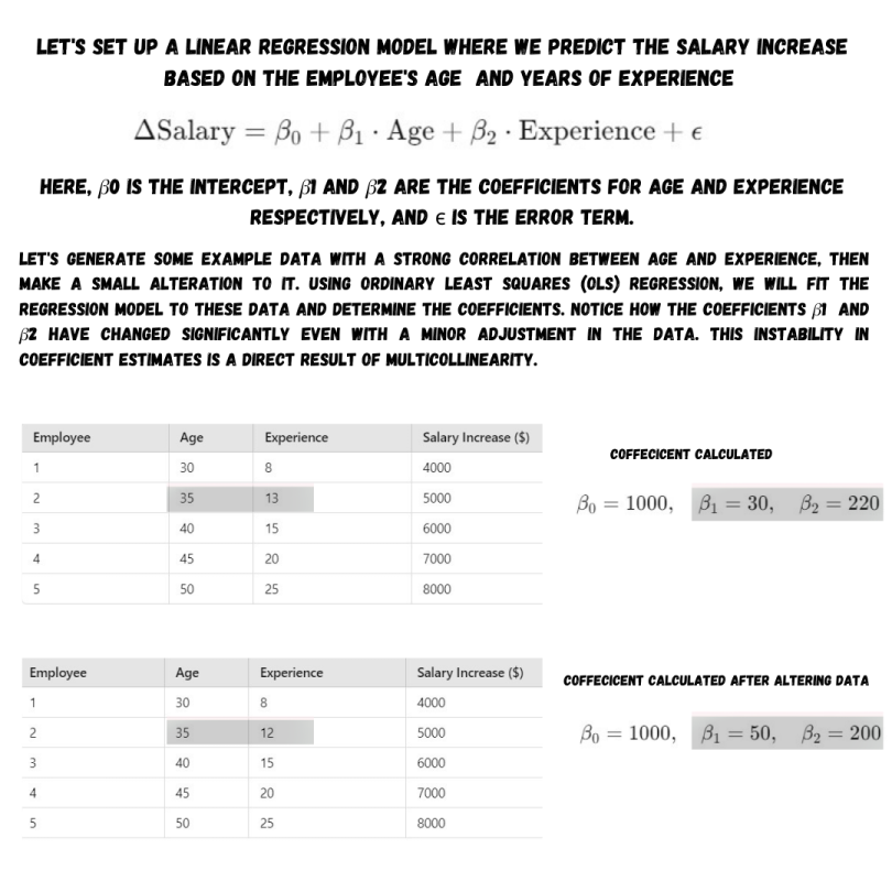
For example, as the employee age increases, years of experience also increase. If most employees start working at a similar age, these two variables will be highly correlated because they provide similar information about the employee’s career length.
The above correlation makes it challenging for the model to separate the impact of age and experience on salary raises. It might lead to inflated standard errors and unstable coefficient estimates, where one couldn’t discern which variable is truly driving changes in salary.
Dummy Variable Multicollinearity
Dummy variable multicollinearity occurs when dummy variables are highly correlated. This usually happens when a category is split into multiple binary variables to be included in a regression model.
Imagine you have a variable for “department” with three categories: human resources, information technology and sales. To include this in your regression model, you create dummy variables like this.
- HR: One if the employee is in HR, zero otherwise.
- IT: One if the employee is in IT, zero otherwise.
- Sales: One if the employee is in sales, zero otherwise.
An employee can only belong to one department at a time. So, by knowing the values of any two dummy variables, you can perfectly predict the department they’re in (e.g., if HR and IT are zero, sales must be one). This perfect linear relationship between dummy variables is a classic case of dummy variable multicollinearity.
Including all dummy variables can lead to perfect multicollinearity, making the regression model unsolvable. To avoid this, you should omit one dummy variable to serve as the reference category.
Here is how you could solve these classic multicollinearity cases. When you encounter structural multicollinearity, reconsider which variables are necessary and avoid redundant ones. For data multicollinearity, consider combining correlated variables or using techniques like principal component analysis to reduce dimensionality. With dummy variable multicollinearity, always omit one category to avoid perfect correlation.
Effects of Multicollinearity
Let’s go back to our employee salary example. Out of all predictors, age and years of experience are major predictors because, typically, as people get older, they also gain more experience.
Considering the above case, here’s how multicollinearity could affect your model.
Unreliable Coefficients
We just established how age and experience go hand in hand, causing multicollinearity. This could lead to coefficient estimates becoming unstable even with minor data variations.
Inflated Standard Errors
Multicollinearity inflates the standard errors of your coefficient estimates. Your coefficient will suggest that both age and experience positively influence salary, but the uncertainty around these estimates increases. This means your model may not reliably pinpoint how much each factor contributes to salary increases.
Misleading Interpretations
Imagine concluding that age significantly impacts salary raises, but it turns out that experience contributes the most. Multicollinearity can blur these distinctions, leading to misleading interpretations, where you could miss observing a strong correlation.
Difficulty in Prediction
When you add data of new employees with varying ages and experiences, multicollinearity can hinder your model’s ability to predict salary raises accurately. The model might struggle to differentiate between the effects of age and experience, potentially leading to less reliable salary predictions.
Identifying and eliminating multicollinearity ensures that your predictions and insights are based on solid statistical reasoning.
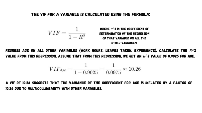
How to Detect Multicollinearity: Variance Inflation Factor (VIF)
Variance Inflation Factor (VIF)
VIF is extensive, measuring the uncertainty (or variance) in one variable’s coefficient because of multicollinearity with others. A high VIF, say above 10, suggests that our model might struggle to separate the effects of correlated variables like age and experience.
To grasp how the VIF works, let’s use a data set involving work hours, age, leaves taken and experience. VIF measures how much the variance (uncertainty) of an estimated regression coefficient increases because of multicollinearity with other variables.
Correlation Matrix
We have a bunch of variables here: work hours, age, leaves taken and experience. A correlation matrix is like a map that shows how strongly these variables are related. With correlation scores, you could identify tightly intertwined variables like age and experience (with correlations around 0.8 or higher).
Refer to the image below for the correlation matrix of our variables, breaking down using a few variables from our data set.
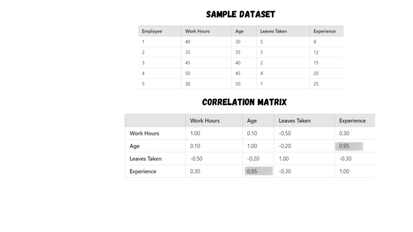
Upon calculating the correlation matrix for these variables, we find that the correlation coefficient of age and experience is very high, which is 0.95, suggesting a strong correlation. Other correlations show weaker associations with low coefficient scores.
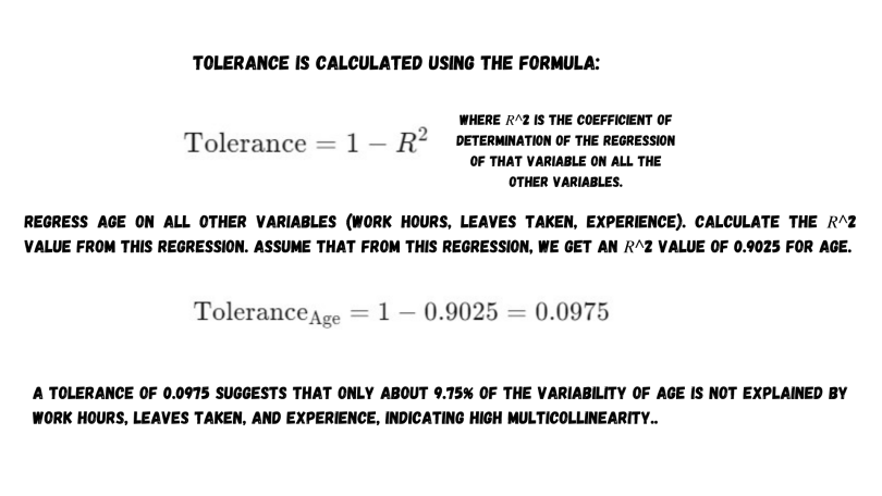
Tolerance
Tolerance is the exact opposite of VIF. It tells us how much information one variable is sharing with others. When tolerance is close to zero, it means that variables are tightly packed together, potentially masking their individual impact on the outcome.
Eigenvalues
This method helps you expose multicollinearity by identifying the variance between two or multiple variables. This redundancy in multicollinearity cases makes certain directions in the data space almost indistinguishable, resulting in very small eigenvalues for those directions.
If a matrix has small eigenvalues, it becomes ill-conditioned, so calculating its inverse requires dividing by these small values. If the most of the eigenvalues are small and are close to zero, it signals multicollinearity.
Consequently, the reciprocals of these eigenvalues, which are part of the inverse matrix, become very large. This inflation of the inverse matrix values then amplifies the variability in the estimated coefficients of the model.
The preceding examples arise in the absence of perfect multicollinearity. Perfect multicollinearity produces a singular matrix for which no inverse matrix exists.
Using the above tools and techniques, we could expose multicollinearity’s tricks in our regression models. The knowledge could help us fine-tune our analyses, ensuring our models paint a clear and accurate picture of how each factor truly influences the outcomes we care about.
How to Fix Multicollinearity
Imagine you’re unraveling the factors influencing employee salary raises, and you’re faced with variables like age and years of experience, two factors that often go hand in hand. Here’s how you can tackle the challenge.
Feature Selection
You shouldn’t include highly correlated variables like age and experience together. Instead, focus on the ingredient (variable) that might have a stronger impact. In this case, factors that might impact salary raises in your industry. An example is tech certifications. This way, your model stays focused and avoids redundancy.
Data Transformation
When you measure variables like years of experience and age differently, it can blur their distinct impacts on salary raises. It requires standardizing or transforming these variables and putting them on a common scale, so the model sees clearer patterns without being bogged down by how they’re measured.
Principal Component Analysis
PCA takes your jumble of correlated variables like age, experience and education and distills them into a few key components. By reducing complexity and focusing on these essential components, PCA helps your model to understand the core influences on salary raises, avoiding the confusion of multicollinearity.
Ridge Regression
Multicollinearity can push coefficients (like age and experience) to unstable extremes. Ridge regression adds balance to these coefficients. It smooths out the bumps caused by correlated variables, ensuring accurate predictions.
Collect More Data
More data broadens your view, capturing diverse scenarios and relationships between predictors. By expanding your data set to include different employee demographics or periods, you bring more variability into play. This wide perspective eliminates multicollinearity and exposes what is behind salary raises across different contexts.
Frequently Asked Questions
Can I ever ignore multicollinearity?
Multicollinearity doesn’t affect the working conditions of a model all the time and can be ignored if you don’t observe prediction errors for a long time.
You can easily ignore multicollinearity when:
- Your model is working well and when you are receiving accurate predictions as expected.
- You don’t want to know the individual contribution of a variable to the outcome, particularly with models like decision trees or random forests. In these cases, there is no linear relationship between variables or variables and outputs.
What level of correlation indicates multicollinearity?
A correlation value of 0.8 or above can be a strong case of multicollinearity requiring attention. Another measure is variance inflation factor (VIF), which is when five or higher than that is a multicollinearity.


