Guide to Expectation Maximization Algorithm

The expectation-maximization (EM) algorithm is an iterative optimization algorithm commonly used in machine learning and statistics to estimate the parameters of probabilistic models, where some of the variables in the model are hidden or unobserved.

The EM algorithm consists of two main steps: the expectation (E) step and the maximization (M) step.

RelatedHow to Make a Python Calculator

What Is the Expectation-Maximization Algorithm?

The expectation-maximization (EM) algorithm is a widely-used optimization algorithm in machine learning and statistics. Its goal is to maximize the expected complete-data log-likelihood, which helps estimate the parameters of probabilistic models where some variables are hidden or unobserved. This approach improves model accuracy by leveraging both observed data and inferred latent structure, even when direct likelihood maximization is intractable.

The EM algorithm is frequently used in clustering, where the assignment of data points to clusters is uncertain or ambiguous. The Gaussian mixture model (GMM) is one of the more popular clustering algorithms that uses the EM algorithm to estimate cluster parameters and assignments.

The EM algorithm is also useful for missing data estimation. The observed data is used to estimate the probability distribution of the missing data, and the algorithm iteratively estimates the missing values. The EM algorithm is also useful for estimating latent variable models like hidden Markov models or hierarchical Bayesian models.

Expectation-Maximization Algorithm Steps

The expectation-maximization algorithm has two main steps: expectation and maximization. It can also include a third step for initialization.

We’ll go over all three steps in the context of a Gaussian mixture model. Specifically, we assume that our data points belong to either of two Gaussian distributions:

1. Initialization

First is the initialization step. We randomly initialize the parameters of the Gaussian distributions: µ₁, σ₁, µ_2, σ₂.

Note: Initialization can affect convergence outcome (e.g. random, K-means++, etc.).

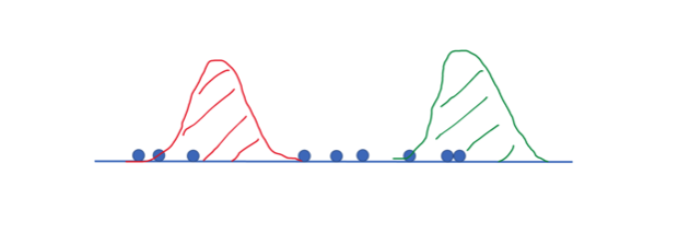
In this illustration, we have nine “missing” data points (z) in one-dimensional space that we believe belong to either of two distributions (red or green). We can do this calculation easily using the probability density functions of the Gaussians.

2. Expectation

Next is the expectation step. Here, we compute the posterior probability that each point belongs to each distribution. This is straightforward using the probability density function:

In our case, we plug in one of our points z₁ for x, and we use either model’s parameters: µ₁ or µ₂ and σ₁ or σ₂ to get relative probabilities that z₁ belongs to either of the two distributions. Then, we compute the posterior responsibilities (or soft assignments) using Bayes’ Theorem for the class probability.

For example, our updated probability that z₁ in the first distribution is:

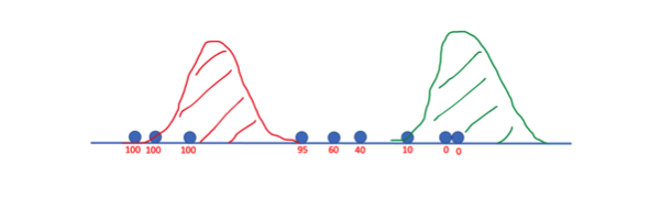
We repeat this process for each data point, resulting in a probability distribution over the two clusters for each point — these are the responsibilities used in the next step.

Here is what the probabilities for belonging to the first distribution might look like:

3. Maximization

Next is the maximization step. Here we update the parameters of the model to maximize the expected log-likelihood, given the responsibilities we just gave our unknown data points.

For the new µ_1, we compute the weighted mean of the data points, where weights are the posterior probabilities of each point belonging to a given Gaussian distribution.

So our new µ₁ is:

Here, r₁ is the probability that z₁ belongs to the first (red) distribution. Remember, this was computed in Step 2. The new σ₁ is similar, we just take the weighted-average squared distance of the points from our new mean. 

We do the same thing for µ₂ and σ₂. Our updated distributions might now look something like this:

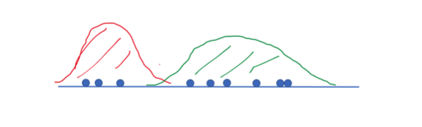
Now, all we do is repeat the expectation and maximization steps until convergence.

Convergence refers to the point at which the algorithm stops iterating because further updates no longer significantly improve the model. In other words, the algorithm has reached a stable solution where the estimated parameters or the log-likelihood of the data no longer change meaningfully between iterations. Convergence in the EM algorithm is typically determined by monitoring how much the model’s parameters or the log-likelihood improve from one iteration to the next. 

And that’s the EM algorithm!

Limitations of the Expectation-Maximization Algorithm

Although the EM algorithm is a powerful statistical tool, it has some limitations.

Doesn’t Always Converge to Global Maximum Likelihood Estimates

One of the main limitations is that it can get stuck in local optima. This means that the algorithm may not always converge to the global maximum likelihood estimates of the parameters.

Assumes Data Is From a Specific Statistical Model

Another limitation is that the algorithm assumes that the data is generated from a specific statistical model, which may not always be the case. For example, we may or may not actually have two Gaussian distributions generating our data but the EM algorithm of course relies on this assumption.

Slow for Large or Complex Data Sets and Models

Finally, the algorithm can be slow for larger data sets and more complicated models.

Frequently Asked Questions