When nothing works, boosting does. Nowadays many people use either XGBoost or LightGBM or CatBoost to win competitions at Kaggle or hackathons. AdaBoost is the first stepping stone in the world of boosting.
3 Facts About AdaBoost:
- The weak learners in AdaBoost are commonly decision trees with a single split, called decision stumps.
- AdaBoost works by putting more weight on difficult to classify instances and less on those already handled well.
- AdaBoost algorithms can be used for both classification and regression problems.
AdaBoost is one of the first boosting algorithms to be adapted in solving practices. AdaBoost helps you combine multiple “weak classifiers” into a single “strong classifier.”
Part 1: Understanding AdaBoost Using Decision Stumps
The power of ensembling is such that we can still build powerful ensemble models even when the individual models in the ensembles are extremely simple.
Decision stumps are the simplest model we could construct in terms of complexity. The algorithm would just guess the same label for every new example, no matter what it looked like. The accuracy of such a model would be best if we guess whichever answer, 1 or 0, is most common in the data. If, say, 60 percent of the examples are 1s, then we’ll get 60 percent accuracy just by guessing 1 every time.
Decision stumps improve upon this by splitting the examples into two subsets based on the value of one feature. Each stump chooses a feature, say X2, and a threshold, T, and then splits the examples into the two groups on either side of the threshold.
To find the decision stump that best fits the examples, we can try every feature of the input along with every possible threshold and see which one gives the best accuracy. While it naively seems like there are an infinite number of choices for the threshold, two different thresholds are only meaningfully different if they put some examples on different sides of the split. To try every possibility, then, we can sort the examples by the feature in question and try one threshold falling between each adjacent pair of examples.
The algorithm just described can be improved further, but even this simple version is extremely fast compared to more complex machine learning models (e.g. training neural networks).
To see this algorithm in action, let’s consider a problem that NFL general managers need to solve: predicting how college wide receivers will do in the NFL. We can approach this as a supervised learning problem by using past players as examples. Here are examples of receivers drafted in 2014. Each one includes some information known about them at the time along with their average receiving yards per game in the NFL from 2014 to 2016:
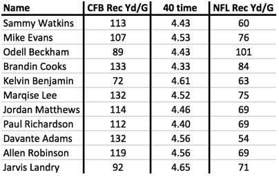
Any application of these techniques to wide receivers would try to predict NFL performance from a number of factors including, at the very least, some measure of the player’s athleticism and some measure of their college performance. Here, I’ve simplified to just one of each: their time in the 40-yard dash (one measure of athleticism) and their receiving yards per game in college.
We can address this as a regression problem, as in the table above, or we can rephrase it as classification by labelling each example as a success (1, orange) or failure (0, blue), based on their NFL production. Here is what the latter looks like after expanding our examples to include players drafted in 2015 as well:
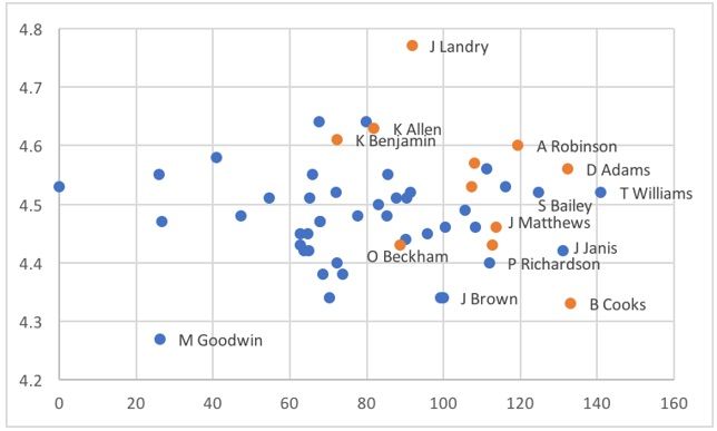
The X-axis shows each player’s college receiving yards per game and the Y-axis shows their 40-time.
Returning to our boosting algorithm, recall that each individual model in the ensemble votes on an example based on whether it lies above or below the model’s threshold for its feature. Here are what the splits look like when we apply AdaBoost and build an ensemble of decision stumps on these data:
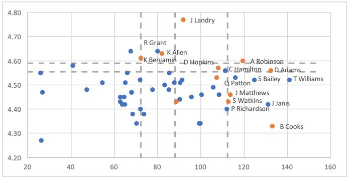
The overall ensemble includes five stumps, whose thresholds are shown as dashed lines. Two of the stumps look at the 40-yard dash (vertical axis), splitting at values between 4.55 and 4.60. The other three stumps look at receiving yards per game in college. Here, the thresholds fall around 70, 90 and 110.
On each side of the split, the stumps will vote with the majority of the examples on that side. For the horizontal lines, there are more successes than failures above the lines and more failures than successes below the lines, so examples with 40-yard dash times falling above these lines will receive “yes” votes from those stumps, while those below the lines get “no” votes. For the vertical lines, there are more successes than failures to the right of the lines and more failures than successes to the left, so examples get “yes” votes for each of the stumps where they fall to the right of the line.
While the ensemble model takes a weighted average of these votes, we aren’t too far off in this case if we imagine the stumps having equal weight. In that case, we would need to get at least three out of five votes to get the majority needed for a successful vote from the ensemble. More specifically, the ensemble predicts success for examples that are above or to the right of at least three lines. The result looks like this:
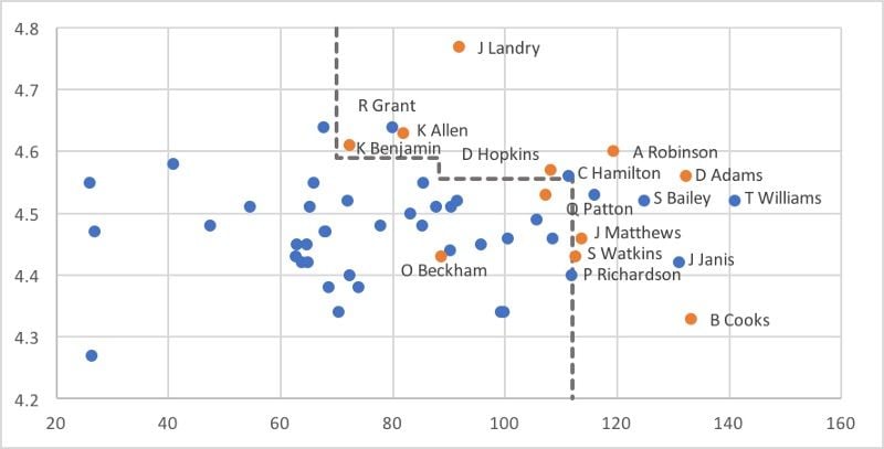
As you can see, this simple model captures the broad shape of where successes appear (and in a non-linear way). It has a handful of false positives, while the only false negative is Odell Beckham Jr., an obvious outlier. As we will see with some investing examples later in the article, the ability to adjust for non-linear relationships between features and outcomes may represent a key advantage over the traditional linear (and logistic) regression used in many investing factor models.
Part 2: Visualizing Ensembles of Decision Stumps
If we have more than two features, then it becomes difficult to visualize the complete ensemble the way we did in the picture above. (It is sometimes said that ML would not be necessary if humans could see in high dimensions.) However, even when there are many features, we can still understand an ensemble of decision stumps by analyzing how it views each individual feature.
To see how, let’s look again at the picture of all the stumps included in the ensemble:
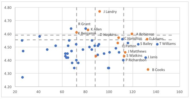
As we see here, there are two stumps that decide based on the 40-yard dash time. If an example has a 40-yard dash time above 4.59, then it receives a success vote from both of these stumps. If it has a time below 4.555, then it receives a “no” vote from both. Finally, if a time falls between 4.55 and 4.59, then it receives a success vote from one stump but not the other. The overall picture looks like this:
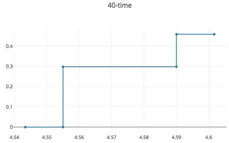
This picture accounts for the fact that the ensemble is a weighted average of the stumps, not a simple majority vote. Those examples with 40-yard dash time above 4.55 get a success vote from the first stump, but that vote has a weight of 0.30. Those with a time above 4.59 get a success vote from the second stump as well, but that stump is only weighted at 0.16, bringing the total weight for a “yes” vote up to 0.46.
As you view this picture and the next, keep in mind that, in order for the model to predict “success” for a new wide receiver, that player would need to accumulate a total weight of at least 0.5.
The picture for the other feature, college receiving yards per game, looks like this:
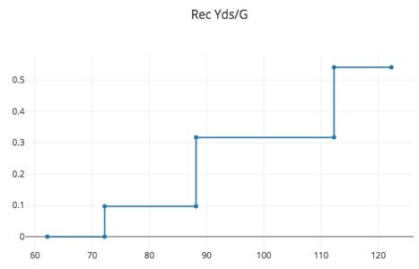
There are three stumps that look at this feature. The first, with a weight of 0.10, votes success on all examples with receiving yards per game at least 72 (or so). The next stump, with a weight of 0.22, votes success on all examples above 88 (or so). Examples with yards above 88 receive success votes from both stumps, giving a weight of at least 0.32 (0.10 plus 0.22). The third stump adds an additional success vote, with the weight of about 0.22 to examples with receiving yards per game above 112 (or so). This brings the total weight of the success votes for those in this range up to about 0.54.
Each of these pictures shows the total weight of success votes that an example will receive from the subset of the ensemble that uses that particular feature. If we group together the individual models into sub-ensembles based on the feature they examine, then the overall model is easily described in terms of these: the total weight of the success votes for example is the sum of the weights from each sub-ensemble, and again if that total exceeds 0.5, then the ensemble predicts the example is a success.
After training a classifier at any level, AdaBoost assigns weight to each training item. Misclassified item is assigned a higher weight so that it appears in the training subset of the next classifier with a higher probability. After each classifier is trained, the weight is assigned to the classifier as well based on accuracy. The more accurate classifier is assigned higher weight so that it will have more impact on the final outcome. A classifier with 50 percent accuracy is given a weight of zero, and a classifier with less than 50 percent accuracy is given a negative weight.
A linear model, in contrast, forces us to make predictions that scale linearly in each parameter. If the weight on some feature is positive, then increasing that feature predicts higher odds of success no matter how high it goes. The ensemble of stumps, which is not bound by that restriction, will not build a model of that shape unless it can find sufficient evidence in the data that this is true. Ensembles of decision stumps generalize linear models, adding the ability to see non-linear relationships between the labels and individual features.
Part 3: Comparing Linear (and Logistic) Regression with AdaBoosting
To see a more realistic example of applying these techniques, we will expand upon the example considered above. In practice, we want to include more information for improved accuracy.
We will add age, vertical jump, weight and absolute numbers of receptions, yards and TDs per game, along with market shares of the team’s totals of those. We will include those metrics from their final college season along with career totals. Altogether, that brings us to a total of 16 features.
Above, we looked at only two years of data. This is still a tiny data set, by any measure, which gives linear models more of an advantage since the risks of overfitting are even larger than usual.
After random splitting data in 8:2 ratio, logistic regression mislabels only 13.7 percent of the training examples. This corresponds to a quite respectable “Pseudo R2” (the classification analogue of R2 for regression) of 0.29. However, on the test set, it mislabels 23.8 percent of the examples. This demonstrates that even when using standard statistical techniques, in-sample error rate is not a good predictor of out-of-sample error.
The model produced by logistic regression has some expected parameter values: receivers are more likely to be successful if they are younger, faster, heavier, and catch more touchdowns. It does not give any weight to vertical jump. On the other hand, it still includes some head scratching parameter values. For example, a larger market share of team receiving yards is good, but a larger absolute number of receiving yards per game is bad. (Perhaps interpretability problems are not unique to machine learning models!)
The ensemble of stumps model improves the error rate from 23.8 percent down to 22.6 percent. While this decrease seems small in the abstract, keep in mind that there are notable draft busts every year, even when decisions are made by NFL GMs who study these players full-time. My guess is that an error rate around 20 percent may be the absolute minimum that we could expect in this setting, so an improvement to 22.6 percent is no small achievement.
Like the logistic regression model, the ensemble of stumps likes wide receivers that are heavier and faster.
With the most important measures of college production, we see some clear non-linearity, which logistic regression has surely missed.
Understanding AdaBoost: Conclusion
As these examples demonstrate, real-world data includes some patterns that are linear but also many that are not. Switching from linear regression to ensembles of decision stumps (aka AdaBoost) allows us to capture many of these non-linear relationships, which translates into better prediction accuracy on the problem of interest, whether that be finding the best wide receivers to draft, the best stocks to purchase or similar machine learning problems.
Frequently Asked Questions
What is AdaBoost?
AdaBoost (Adaptive Boosting) is a machine learning algorithm and boosting technique that combines multiple weak classifiers, typically decision stumps, into a single strong classifier. It works by reweighting training data to focus on hard-to-classify examples and assigning more influence to accurate classifiers.
What are decision stumps and why are they used in AdaBoost?
Decision stumps are simple models that split data using a single feature and threshold. AdaBoost uses them as weak learners because they are fast to train and can be combined to capture complex patterns.
Can AdaBoost be used for both classification and regression?
Yes, AdaBoost can handle both classification and regression tasks, though its use in classification is more common and well-documented.


