

Graph theory is the study of relationships. Given a set of nodes and connections, which can abstract anything from city layouts to computer data, graph theory provides a helpful tool to quantify and simplify the many moving parts of dynamic systems.
This might sound like an intimidating and abstract concept. While it might not seem like a theory that has any application, there are actually an abundance of useful and important applications of graph theory. In this article, I’ll briefly explain what some of these applications are and do my best to convince you that having some basic knowledge can be useful to solve some interesting problems you might come across.
What Is Graph Theory?
Graph Theory is the study of relationships, providing a helpful tool to quantify and simplify the moving parts of a dynamic system. It allows researchers to take a set of nodes and connections that can abstract anything from city layouts to computer data and analyze optimal routes. It’s used in social network connections, ranking hyperlinks in search engines, GPS maps to find the shortest route home, and more.
I’ll go over an example and show you how a route planning/optimization task can be formulated and solved using graph theory. More specifically, I’ll consider a large warehouse consisting of 1,000s of different items in various locations/pickup points. The challenge here is, given a list of items, which path should you follow through the warehouse to pick up all items, and at the same time, minimize the total distance traveled? For those of you familiar with these kinds of problems, this resembles the famous traveling salesman problem, a well known problem in combinatorial optimization that’s important in theoretical computer science and operations research.
My aim isn’t to give a comprehensive introduction to graph theory, which would be a tremendous task. Rather, through a real-world example, I plan to convince you that knowing at least the basics of graph theory can prove to be very useful.
Let’s start with a brief historical introduction to the field of graph theory and highlight the importance and the wide range of useful applications in many vastly different fields. Following this more general introduction, I will then shift focus to the warehouse optimization example discussed above.
The History of Graph Theory
Graph theory was first introduced in the 18th century by the Swiss mathematician Leonhard Euler. His work on the famous “Seven Bridges of Königsberg problem,” is considered the origin of graph theory.
The city of Königsberg in Prussia (present-day Kaliningrad, Russia) was set on both sides of the Pregel River and included two large islands — Kneiphof and Lomse — that were connected to each other via the two mainland portions of the city by seven bridges. The problem was to devise a walk through the city that would cross each of those bridges once and only once.
Euler, recognizing that the relevant constraints were the four bodies of land and the seven bridges, drew out the first known visual representation of a modern graph. A modern graph, as seen in the bottom-right image, is represented by a set of points known as vertices or nodes, connected by a set of lines known as edges.
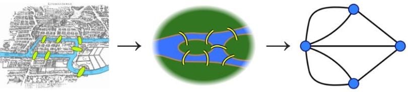
This abstraction from a concrete problem concerning a city and bridges to a graph makes the problem tractable mathematically, as this abstract representation includes only the information important for solving the problem. Euler actually proved that this specific problem has no solution. However, the challenge he faced was the development of a suitable technique of analysis and subsequent tests established this assertion with mathematical rigor. From there, the branch of math known as graph theory lay dormant for decades. In modern times, however, its applications are finally exploding.
How Graph Theory Is Used
Let’s go over some of the basics of graph theory as it pertains to different kinds of graphs. This will be of relevance to the example we’ll discuss later on path optimization.
Because graph theory is the study of relationships, it provides a helpful tool for quantifying and simplifying the many moving parts of dynamic systems. Studying graphs through a framework provides answers to many arrangement, networking, optimization, matching and operational problems.
Graphs can be used to model many types of relations and processes in physical, biological, social and information systems, and it has a wide range of useful applications, such as:
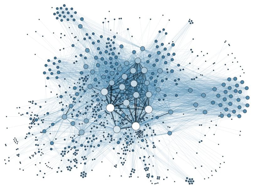
- Finding communities in networks, such as social media (friend/connection recommendations), or for possible spread of COVID-19 in the community through contacts.
- Ranking hyperlinks in search engines.
- GPS in Google maps to find the shortest path home.
- Study of molecules and atoms in chemistry.
- DNA sequencing.
- Computer network security.
There are several types of graphs that describe different kinds of problems and the constraints within them.
Types of Graphs
There are many different kinds of graph representations. When solving a problem that includes graphs, we first need to determine what kind of graph we’re dealing with.
3 Types of Graphs to Know in Graph Theory
- Undirected graphs: All paths between each node are bidirectional.
- Directed graphs (digraphs): Paths between the nodes have specified directions.
- Weighted graphs: The paths between each node have specified directions and weights to indicate distance.
Undirected Graphs
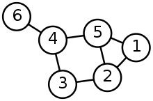
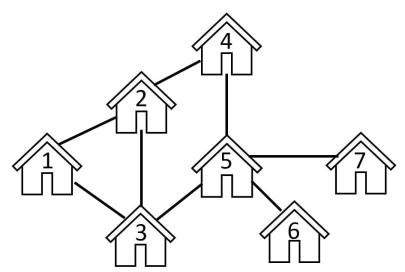
In an undirected graph, let each node of the network represent houses at different locations in a city and the edges as the roads between them. As the name implies, there isn’t a specified direction between the nodes of the graph. This means that an edge (road) connecting nodes (houses) 1-to-2 would be identical to the edge from 2-to-1.
In this initial example, we assumed that all roads are bidirectional and that we don’t need to worry about any one-way streets.
Directed Graphs (DiGraphs)
When we’re dealing with directed graphs, we also need to specify the direction between the different nodes. This means that if you have an edge from node 1-to-2, this does not necessarily mean that you can also move in the opposite direction from 2-to-1.
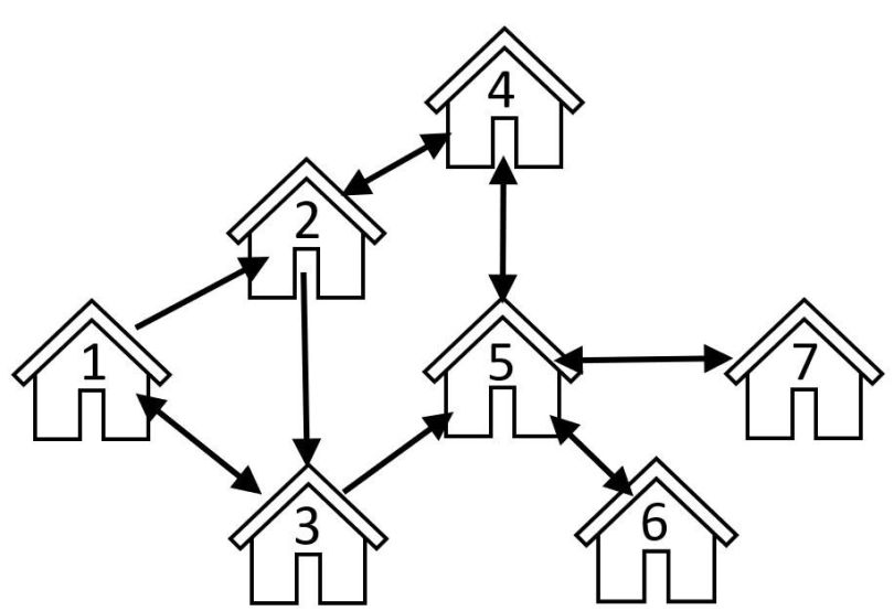
If we stick to the previous example of nodes representing houses at different locations in a city, this means that if we have a directed edge from 1-to-2 we have a one-way street between those houses. We can then drive from house 1-to-2, but driving the opposite direction from 2-to-1 would not be permitted. We would need to take the route 2-to-3-to-1. However, between houses 2 and 4, we can safely drive in either direction, as indicated by the double arrows.
Weighted Graphs
In many real-world applications, we would also need to associate a “weight” to the edges of our graph to represent implications such as cost, distance, etc.
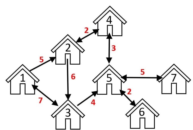
Weighted graphs can either be directed or undirected. If we keep to the same example of roads connecting houses in a city, the weight of the edges could in this case represent the driving distance between them. For example, if we want to find the optimal route from the “House 1” on the left to “House 5,” we’d need to consider both the possible driving routes (edges), as well as the distances (edge weights).
In this case, this means that the optimal route would be 1-to-2-to-4-to-5, where the total distance would be 5+2+3=10, rather than the other possible route 1-to-3-to-5, where the distance would be 7+4=11.
Based on this simple example, you can probably imagine that the use of weighted graphs is applicable to many real-world scenarios, for example route planning, search engines comparing flight times and cost, planning the optimal layout of road networks and infrastructure in cities, etc.
It’s now time to focus on our example case of route planning when picking items in our warehouse.
Graph Theory Use Case: Warehouse Pickup Route Optimization
Given a picking list as input, we need to find the shortest route that both passes all the pickup points and also complies to route restrictions with regard to where it’s possible to drive. The assumptions and constraints here are that crossing between corridors in the warehouse is only allowed at marked “turning points.” Also, the direction of travel must follow the specified legal driving direction for each corridor.
Solution
This problem can be formulated as an optimization problem in graph theory. All pick up points in the warehouse form a “node” in the graph, where the edges represent permitted lanes/corridors and distances between the nodes. To introduce the problem more formally, let’s start with a simple example.
The graph below represents two corridors with five shelves/pickup points per corridor. All shelves are represented as a node in the graph with an address ranging from one to 10. The arrows indicate the permitted driving direction, where the double arrows indicate that you can drive either way. Simple enough, right?
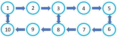
Being able to represent the permitted driving routes in the form of a graph, means that we can use mathematical techniques known from graph theory to find the optimal “driving route” between the nodes (i.e., the stock shelves in our warehouse).
The example graph can be described mathematically through an adjacency matrix. The adjacency matrix to the right in the below figure is thus a representation of our warehouse graph, which indicates all permitted driving routes between the various nodes.
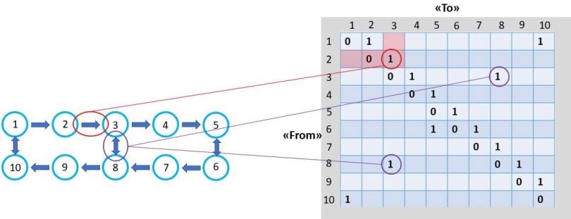
- Example 1: You are allowed to travel from node 2 → 3, but not from 3 → 2. This is indicated by the “1” in the adjacency matrix to the right.
- Example 2: You are allowed to go from both node 8 → 3, and from 3 → 8, again indicated by the “1”’s in the adjacency matrix, which in this case is symmetric when it comes to travel direction.
Back to the Warehouse Problem
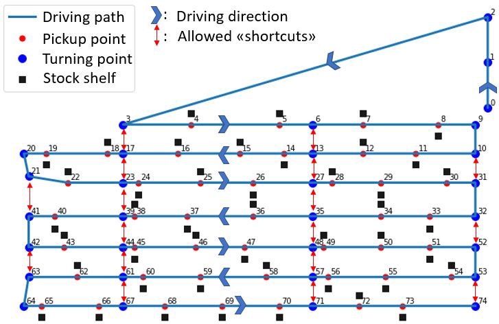
A real warehouse is bigger and more complex than the above example. However, the main principles of how to represent the problem through a graph remains the same. To make the problem slightly simpler, and more visually suitable for this article, I reduced the total number of shelves/pickup-points to approximately every 50th shelf, marked with black squares in the figure below. All pickup points are given an address, a node number, from one to 74. The other relevant constraints mentioned earlier, such as permitted driving directions in each of the corridors as well as the allowed “turning points” and shortcuts between the corridors, are also indicated in the figure.
The next step is to represent this graph in the form of an adjacency matrix. Since we are interested in finding both the optimal route and total distance, we must also include the driving distance between the various nodes in the matrix.
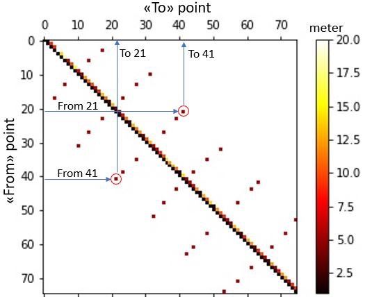
This matrix indicates all constraints with regard to the permitted travel direction, which “shortcuts” are permitted, any other restrictions, as well as the driving distance between the nodes illustrated through color. As an example, the shortcut between nodes 21 and 41 shown in the graph representation can also be identified in the adjacency matrix. The “white areas” of the matrix represent the paths that aren’t allowed, indicated through an “infinite” distance between those nodes.
How to Use Graph Theory for Path Optimization
An an abstracted representation of our warehouse in the form of a graph doesn’t solve our actual problem. The idea is that through this graph representation, we can now use the mathematical framework and algorithms from graph theory to solve it.
Since graph optimization is a well-known field in mathematics, there are several methods and algorithms that can solve this type of problem. In this example, I have based the solution on the Floyd-Warshall algorithm, which is a well known algorithm for finding shortest paths in a weighted graph. A single execution of the algorithm will find the lengths (summed weights) of shortest paths between all pairs of nodes. Although it doesn’t return details of the paths themselves, it is possible to reconstruct the paths with simple modifications to the algorithm.
If you give this algorithm as input a “picking order list,” in which you go through a list of items you want to pick, you should be able to obtain the optimal route that minimizes the total driving distance to collect all items on the list.
Graph Theory Path Optimization Example
Let’s start by visualizing the results for a (short) picking list as follows: Start at node 0 then pick up items at nodes 15, 45, 58 and 73 (these locations are illustrated in the figure below).
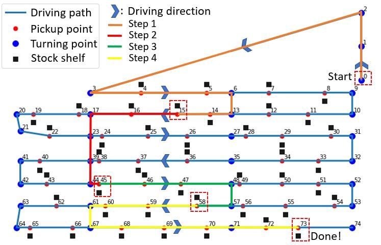
The algorithm finds the shortest allowable route between these points through calculating the “distance matrix,” D, which can then be used to determine the total driving distance between all locations/nodes in the picking list.
- Step 1:
D[0][15] → 90 m - Step 2:
D[15][45] →52 m - Step 3:
D[45][58] → 34 m - Step 4:
D[58][73] → 92 m
Total distance = 268m.
Having tested several picking lists as input and verifying the proposed driving routes and calculated distance, the algorithm is able to find the optimal route in all cases. The algorithm respects all the imposed constraints, such as the permitted direction of travel and uses all permitted “shortcuts” to minimize the total distance.
From Path Optimization to Useful Insights
We’ve now developed an optimization algorithm that calculates the optimal driving route via all points on a picking order list for a simplified version of the warehouse. By providing a list of picking orders as input, one can relatively easily calculate statistics on typical mileage per picking order. These statistics can then be filtered on various information such as item type, customer, date, etc. In the following section, I’ve picked a few examples on how one can extract interesting statistics from such a path optimization tool.
I first generated 10,000 picking order lists where the number of items per list ranges from one to 30 items, located at random pickup points in the warehouse (address three to 74 in the previous figure above). we can perform the path optimization procedure over all of these picking lists to extract some interesting statistics.
Optimizing the Number of Items in a Pickup Order
Calculate mileage as a function of the number of units per picking order list. You would naturally assume that the total mileage increases the more items you have to pick. But, at some level, this will start to flatten out. This is due to the fact that one eventually has to stop by all the corridors in the warehouse to pick up goods, which then prevents us from making use of clever “shortcuts” to minimize the total driving distance.
This tendency can be illustrated in the figure below to the left, which illustrates that for more than approximately 15-to-20 units per picking order, adding extra items doesn’t make the total mileage much longer. You have to drive through all corridors of the warehouse anyway. Note that the figures show a “density plot” of the distribution of typical mileage per picking orders list.
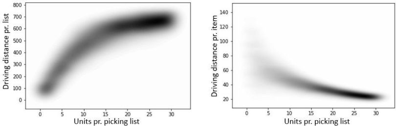
Another interesting statistic, which shows the same trend, is the distribution of driving distance per picked item in the figure to the right. We see that for picking lists with few items, the typical mileage per item is relatively high, with a large variance, depending on how “lucky” we are with some items being located in the same corridor, etc. For picking lists with several items, the mileage per item gradually decreases. This type of statistic can thus be interesting to investigate closer in order to optimize how many items each picking order list should contain in order to minimize the mileage per picked item.
Mileage Per Order
I’ve used real-world data that also contains additional information in the form of a customer ID, shown for only two customers. We can then take a closer look at the distribution in mileage per picking order list for the two customers. For example, do you typically have to drive longer distances to pick the goods of one customer versus another? And, should you charge that customer extra for this additional cost?
The left-most figure below shows the distribution in mileage for Customer 1 and Customer 2, respectively. One of the things we can interpret from this is that for customer 2, most picking order lists have a noticeably shorter driving distance compared to customer 1. This can also be shown by calculating the average mileage per picking order list for the two customers (figure to the right).
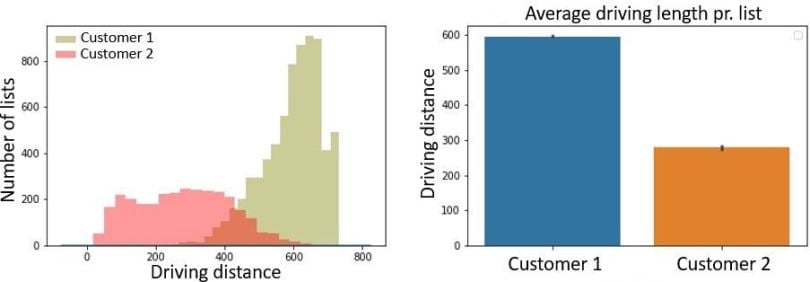
This type of information can be used to implement pricing models where the product price to the customer is also based on mileage per order. For customers where the order involves more driving, and thus also more time and higher cost), you can consider invoicing extra compared to orders that involve short driving distances.
Why Graph Theory is Important
I hope I’ve convinced you that graph theory isn’t just some abstract mathematical concept but one that actually has many useful and interesting applications. Hopefully, the examples above will be useful for solving similar problems later on, or at least satisfying some of your curiosity when it comes to graph theory and its applications.