How to Beautify Your Matplotlib Histograms

Histograms are the most common method for visualizing the distribution of a variable. A simple histogram can be very useful to get a first glance at the data. However, compared to other prominent plot types like pie, bar or line plots, they’re rather boring to look at. Most importantly, they require a statistical background to be interpreted correctly. 

However, before we ditch the histogram entirely, let’s try and make it more beautiful, richer in information as well as easier to interpret.

In this tutorial, we’ll take a standard Matplotlib histogram and improve it aesthetically as well as add some useful components. For this, we’ll follow a three-step-procedure:

1. Add Information
2. Remove Information
3. Emphasize Information

 

How to Build a Simple Histogram in Matplotlib

For this article, we’ll use the “Avocado Prices” data set from Kaggle. Price distributions in a market are a useful application for histograms.

We only need these two libraries for this:

import pandas as pd
import matplotlib.pyplot as plt

Because we only need one column (“AveragePrice”), we can read the data as a series instead of as a dataframe. That way, we’ll save the time to specify columns later on.

avocado = pd.read_csv("avocado.csv")["AveragePrice"]

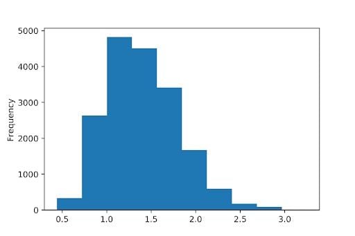
Our first and very basic histogram can be plotted very easily using this code:

fig, ax = plt.subplots(figsize = (6,4))
avocado.plot(kind = "hist")
plt.show()

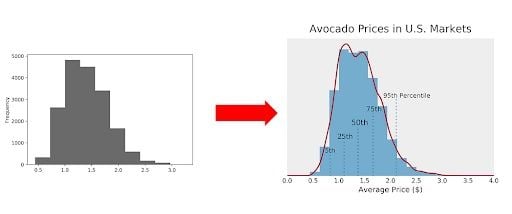
After following the three steps of this tutorial, we’ll get this end result:

Let’s get started.

More on Data Science8 Data Visualization Tools That Every Data Scientist Should Know

 

3 Steps to Beautify Matplotlib Histograms

Below are three steps to improving your histograms using Matplotlib.

 

1. Add Information

An obvious thing to add would be the title and axes labels. If you compare the two figures above, you’ll find that the histogram is much less “blocky” in the second plot. We can achieve this by increasing the number of bins, which is essentially the number of classes the histogram divides the data into. More bins will make the histogram smoother. 

Finally, you’ve likely noticed that the second figure has a line around the histogram. This line is called a kernel-density-estimation (KDE). KDE tries to compute the underlying distribution of a variable, which will draw a very smooth line around the histogram. However, KDE will only work if we change the y axis from absolute values to density values. The downside to this is that density values are a challenge to interpret for most people. We’ll fix that issue later. First, let’s code this:

fig, ax = plt.subplots(figsize = (6,4))

# Plots #
    # Plot histogram
avocado.plot(kind = "hist", density = True, bins = 15) # change density to true, because KDE uses density
    # Plot KDE
avocado.plot(kind = "kde")

# X #
ax.set_xlabel("Average Price ($)")

# Y #
ax.set_ylim(0, 1)

# Overall #
ax.set_title("Avocado Prices in U.S. Markets")

plt.show()

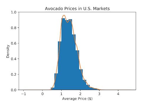
We can see that the visualization is now richer in information. However, it’s not exactly beautiful and a bit overwhelming. Let’s reduce the amount of information to make the plot cleaner.

 

2. Remove Information

Some of the information in the last figure is irritating or even completely useless. For example, the y axis is not interpretable anymore for most people. We should remove the ticks and tick labels and label the axis with “Frequency” again. This will give the reader an idea of what the axis means without confusing them with unnecessary numbers. 

Furthermore, the KDE has estimated the density for values under $0. Obviously, we need to fix that by rescaling the x axis. In most cases, you can remove any ticks and spines in a plot without losing much readability. Let’s apply all of this:

fig, ax = plt.subplots(figsize = (6,4))

# Plots #
    # Plot histogram
avocado.plot(kind = "hist", density = True, bins = 15) # change density to true, because KDE uses density
    # Plot KDE
avocado.plot(kind = "kde")

# X #
ax.set_xlabel("Average Price ($)")
    # Limit x range to 0-4 
ax.set_xlim(0, 4)

# Y #
ax.set_ylim(0,1)
    # Remove y ticks
ax.set_yticks([])
    # Relabel the axis as "Frequency"
ax.set_ylabel("Frequency")

# Overall #
ax.set_title("Avocado Prices in U.S. Markets")
# Remove ticks and spines
ax.tick_params(left = False, bottom = False)
for ax, spine in ax.spines.items():
    spine.set_visible(False)
    
plt.show()

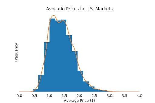
This looks much cleaner already. In the last step, we can emphasize specific information and make aesthetic improvements.

More on Data Science7 Ways to Tell Powerful Stories With Your Data Visualization

 

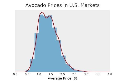
3. Emphasize Information

Emphasizing information doesn’t just mean increasing font sizes, but also, for example, choosing a color scheme that is beneficial to the message you are trying to convey with your visualization. Since this step will take a lot more code, I’ll show code snippets separately.

First, we need a different set of colors. The orange/blue combination in the previous plots just doesn’t look good. An easy way to change your plots layout is to change the matplotlib style sheet. Personally, I love the “bmh” style sheet. However, this style sheet adds a grid, which would be distracting in our plot. Let’s change the style sheet to “bmh” and remove the grid it produces.

plt.style.use("bmh")
# Later in the code
ax.grid(False)

Another aesthetic improvement would be to reduce the histogram opacity. This will make the KDE more dominant, which will give the reader an overall smoother impression.

avocado.plot(kind = "hist", density = True, alpha = 0.65, bins = 15) 

To make the title stand out more, we can increase its font size. The “pad” argument will allow us to add an offset, too.

ax.set_title("Avocado Prices in U.S. Markets", size = 17, pad = 10)

During this step, I also wondered whether the y label “Frequency” was necessary. After testing both variants, I found having a y label more confusing than helpful. If no other information is given, I think we intuitively read the y axis as “Frequency”.

ax.set_ylabel("")

If we applied all of the above, we would get this plot:

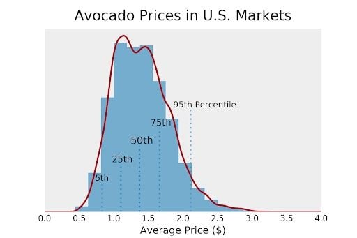
At this point, the visualization is ready for your presentation or report. However, there is one more thing we could do to make the plot more interpretable. In principle, histograms hold all the information we need to display percentiles. Unfortunately, it’s impossible to read the information directly from the plot. 

What if we want to show our boss what the 75th percentile of avocado prices is while keeping all the information about the distribution? We could compute some percentiles and display them in the plot as vertical lines. This is similar to what a boxplot would do but actually integrated into the histogram. Let’s try this.

First, we want to plot the vertical lines. For this, we’ll calculate the fifth, 25th, 50th, 75th, and 95th percentiles of the distribution. One way to do it would be to make every vertical line a bit longer than the previous one in a kind of stepwise motion. We can also give the inner lines a higher opacity than the outer lines.

To do this, we’ll store the quantiles, line opacities and line lengths in a list of lists. This will allow us to loop through this list and plot all lines automatically.

# Calculate percentiles
quant_5, quant_25, quant_50, quant_75, quant_95 = avocado.quantile(0.05), avocado.quantile(0.25), avocado.quantile(0.5), avocado.quantile(0.75), avocado.quantile(0.95)

# [quantile, opacity, length]
quants = [[quant_5, 0.6, 0.16], [quant_25, 0.8, 0.26], [quant_50, 1, 0.36],  [quant_75, 0.8, 0.46], [quant_95, 0.6, 0.56]]

# Plot the lines with a loop
for i in quants:
    ax.axvline(i[0], alpha = i[1], ymax = i[2], linestyle = ":")

Now, we need to add labels. Just like before, we can use different opacities, and in this case, font sizes to reflect the density of the distribution. Each text should have a little offset compared to the percentile lines for better readability.

ax.text(quant_5-.1, 0.17, "5th", size = 10, alpha = 0.8)
ax.text(quant_25-.13, 0.27, "25th", size = 11, alpha = 0.85)
ax.text(quant_50-.13, 0.37, "50th", size = 12, alpha = 1)
ax.text(quant_75-.13, 0.47, "75th", size = 11, alpha = 0.85)
ax.text(quant_95-.25, 0.57, "95th Percentile", size = 10, alpha =.8)

We can now use this histogram to make business decisions on at which price to sell our avocados. Maybe our avocados are a bit better than the average avocado and our company is rather well-known for their avocados. Maybe we should charge the price that is at the 75th percentile of the distribution (around $1.65)? This histogram is a combination of histogram and boxplot, in a way.

fig, ax = plt.subplots(figsize = (6,4))

# Plot
    # Plot histogram
avocado.plot(kind = "hist", density = True, alpha = 0.65, bins = 15) # change density to true, because KDE uses density
    # Plot KDE
avocado.plot(kind = "kde")

    # Quantile lines
quant_5, quant_25, quant_50, quant_75, quant_95 = avocado.quantile(0.05), avocado.quantile(0.25), avocado.quantile(0.5), avocado.quantile(0.75), avocado.quantile(0.95)
quants = [[quant_5, 0.6, 0.16], [quant_25, 0.8, 0.26], [quant_50, 1, 0.36],  [quant_75, 0.8, 0.46], [quant_95, 0.6, 0.56]]
for i in quants:
    ax.axvline(i[0], alpha = i[1], ymax = i[2], linestyle = ":")


# X
ax.set_xlabel("Average Price ($)")
    # Limit x range to 0-4
x_start, x_end = 0, 4
ax.set_xlim(x_start, x_end)

# Y
ax.set_ylim(0, 1)
ax.set_yticklabels([])
ax.set_ylabel("")

# Annotations
ax.text(quant_5-.1, 0.17, "5th", size = 10, alpha = 0.8)
ax.text(quant_25-.13, 0.27, "25th", size = 11, alpha = 0.85)
ax.text(quant_50-.13, 0.37, "50th", size = 12, alpha = 1)
ax.text(quant_75-.13, 0.47, "75th", size = 11, alpha = 0.85)
ax.text(quant_95-.25, 0.57, "95th Percentile", size = 10, alpha =.8)

# Overall
ax.grid(False)
ax.set_title("Avocado Prices in U.S. Markets", size = 17, pad = 10)

    # Remove ticks and spines
ax.tick_params(left = False, bottom = False)
for ax, spine in ax.spines.items():
    spine.set_visible(False)
    
plt.show()

And that’s the entire code for the final histogram.