Neural networks are good at almost every task but they rely on more and more data to perform well. For certain problems like facial recognition and signature verification, we can’t always rely on getting more data. To solve these kinds of tasks we have a new type of neural network architecture called Siamese networks.
What Are Siamese Networks?
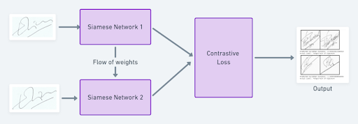
A Siamese neural network (SNN) is a class of neural network architectures that contain two or more identical sub-networks (which have the same configuration with the same parameters and weights).
Siamese networks are able to use only a few images to get better predictions. The ability to learn from very little data has made Siamese networks more popular in recent years. In this article, I’ll show you what Siamese networks are and how to develop a signature verification system with PyTorch using Siamese networks.
What Are Siamese Networks?

A Siamese neural network (SNN) is a class of neural network architectures that contain two or more identical sub-networks. “Identical” here means they have the same configuration with the same parameters and weights. Parameter updating is mirrored across both sub-networks and it’s used to find similarities between inputs by comparing its feature vectors. These networks are used in many applications.
Traditionally, a neural network learns to predict multiple classes. This poses a problem when we need to add or remove new classes to the data. In this case, we have to update the neural network and retrain it on the whole data set. Also, deep neural networks need a large volume of data on which to train. SNNs, on the other hand, learn a similarity function. Thus, we can train the SNN to see if two images are the same (which I’ll demonstrate below). This process enables us to classify new classes of data without retraining the network.
How to Train a Siamese Network
- Initialize the network, loss function and optimizer.
- Pass the first image of the pair through the network.
- Pass the second image of the pair through the network.
- Calculate the loss using the outputs from the first and second images.
- Backpropagate the loss to calculate the gradients of our model.
- Update the weights using an optimizer.
- Save the model.
Pros and Cons of Siamese Networks
Siamese Network Pros
More Robust to Class Imbalance
Giving a few images per class is sufficient for Siamese networks to recognize those images in the future with the aid of one-shot learning.
Nice to Pair With the Best Classifier
Given that an SNN’s learning mechanism is somewhat different from classification models, simply averaging it with a classifier can do much better than averaging two correlated supervised models (e.g. GBM & RF classifiers).
Learning from Semantic Similarity
SNN focuses on learning embeddings (in the deeper layer) that place the same classes/concepts close together. Hence, we can learn semantic similarity.
Siamese Network Cons
Needs More Training Time Than Normal Networks
Since SNNs involves learning from quadratic pairs (to see all information available) they’re slower than the normal classification type of learning (pointwise learning).
Don’t Output Probabilities
Since training involves pairwise learning, SNNs don’t output class probabilities. Instead, they return a similarity score (like a distance metric) between two inputs.
Loss Functions Used in Siamese Networks

Since training SNNs involve pairwise learning, cross entropy loss cannot be used. Instead, there are two distance-based loss functions we typically use to train Siamese networks: triplet loss or contrastive loss.
Triplet Loss
Triplet loss is a loss function where we compare a baseline (anchor) input to a positive (truthy) input and a negative (falsy) input. The distance from the baseline (anchor) input to the positive (truthy) input is minimized, and the distance from the baseline (anchor) input to the negative (falsy) input is maximized.
In the above equation, alpha is a margin term used to stretch the distance between similar and dissimilar pairs in the triplet. Fa, Fp, Fn are the feature embeddings for the anchor, positive and negative images.
During the training process, we feed an image triplet (anchor image, negative image, positive image)(anchor image, negative image, positive image) into the model as a single sample. The distance between the anchor and positive images should be smaller than that between the anchor and negative images.
Contrastive Loss
Contrastive loss is an increasingly popular loss function. It’s a distance-based loss as opposed to more conventional error-prediction loss. This loss function is used to learn embeddings in which two similar points have a low Euclidean distance and two dissimilar points have a large Euclidean distance.

We define Dw (the Euclidean distance) as:

Gw is the output of our network for one image.
Signature Verification With Siamese Networks

As Siamese networks are mostly used in verification systems (face recognition, signature verification, etc.), let’s implement a signature verification system using Siamese neural networks in PyTorch.
Data Set and Preprocessing the Data Set

We are going to use the ICDAR 2011 data set which consists of genuine and fraudulent Dutch signatures. The data set itself is separated as train and folders. Inside each folder, it consists of files separated as genuine and forgery. The data set also contains the labels as CSV files. You can download the data set here.
To feed this raw data into our neural network, we have to turn all the images into tensors and add the labels from the CSV files to the images. To do this we can use the custom data set class from PyTorch.
Here’s what our full code will look like:
#preprocessing and loading the data set
class SiameseDataset():
    def __init__(self,training_csv=None,training_dir=None,transform=None):
        # used to prepare the labels and images path
        self.train_df=pd.read_csv(training_csv)
        self.train_df.columns =["image1","image2","label"]
        self.train_dir = training_dir
        self.transform = transform

    def __getitem__(self,index):
        # getting the image path
        image1_path=os.path.join(self.train_dir,self.train_df.iat[index,0])
        image2_path=os.path.join(self.train_dir,self.train_df.iat[index,1])
        # Loading the image
        img0 = Image.open(image1_path)
        img1 = Image.open(image2_path)
        img0 = img0.convert("L")
        img1 = img1.convert("L")
        # Apply image transformations
        if self.transform is not None:
            img0 = self.transform(img0)
            img1 = self.transform(img1)
        return img0, img1 , th.from_numpy(np.array([int(self.train_df.iat[index,2])],dtype=np.float32))
    def __len__(self):
        return len(self.train_df)
After preprocessing the data set, we have to load the data set into PyTorch using the DataLoader class. We’ll use the transform function to reduce the image size into 105 pixels of height and width for computational purposes.
# Load the the dataset from raw image folders
siamese_dataset = SiameseDataset(training_csv,training_dir,
                                        transform=transforms.Compose([transforms.Resize((105,105)),
                                                                      transforms.ToTensor()
                                                                      ])
                                      )
Neural Network Architecture
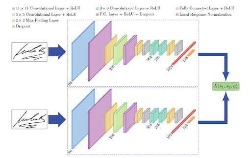
Now let’s create a neural network in PyTorch. We’ll use the neural network architecture which will be similar, as described in the SigNet paper.
#create a siamese network
class SiameseNetwork(nn.Module):
    def __init__(self):
        super(SiameseNetwork, self).__init__()
        # Setting up the Sequential of CNN Layers
        self.cnn1 = nn.Sequential(
            nn.Conv2d(1, 96, kernel_size=11,stride=1),
            nn.ReLU(inplace=True),
            nn.LocalResponseNorm(5,alpha=0.0001,beta=0.75,k=2),
            nn.MaxPool2d(3, stride=2),

            nn.Conv2d(96, 256, kernel_size=5,stride=1,padding=2),
            nn.ReLU(inplace=True),
            nn.LocalResponseNorm(5,alpha=0.0001,beta=0.75,k=2),
            nn.MaxPool2d(3, stride=2),
            nn.Dropout2d(p=0.3),

            nn.Conv2d(256,384 , kernel_size=3,stride=1,padding=1),
            nn.ReLU(inplace=True),

            nn.Conv2d(384,256 , kernel_size=3,stride=1,padding=1),
            nn.ReLU(inplace=True),
            nn.MaxPool2d(3, stride=2),
            nn.Dropout2d(p=0.3),
        )
        # Defining the fully connected layers
        self.fc1 = nn.Sequential(
            nn.Linear(30976, 1024),
            nn.ReLU(inplace=True),
            nn.Dropout2d(p=0.5),

            nn.Linear(1024, 128),
            nn.ReLU(inplace=True),

            nn.Linear(128,2))

    def forward_once(self, x):
        # Forward pass
        output = self.cnn1(x)
        output = output.view(output.size()[0], -1)
        output = self.fc1(output)
        return output

    def forward(self, input1, input2):
        # forward pass of input 1
        output1 = self.forward_once(input1)
        # forward pass of input 2
        output2 = self.forward_once(input2)
        return output1, output2
In the above code, we have created our network as follows:
-
The first convolutional layers filter the
105*105input signature image with 96 kernels of size 11 with a stride of one pixel. -
The second convolutional layer takes as input the (response-normalized and pooled) output of the first convolutional layer and filters it with 256 kernels of size five.
-
The third and fourth convolutional layers are connected to one another without any intervention of pooling or normalization of layers. The third layer has 384 kernels of size three connected to the (normalized, pooled and dropout) output of the second convolutional layer. The fourth convolutional layer has 256 kernels of size three.
This leads to the neural network learning fewer lower-level features for smaller receptive fields and more features for higher-level or more abstract features.
The first fully connected layer has 1024 neurons, whereas the second fully connected layer has 128 neurons. This indicates that the highest learned feature vector from each side of SigNet has a dimension equal to 128.
So where is the other network?
Since the weights are constrained to be identical for both networks, we use one model and feed it two images in succession. After that, we calculate the loss value using both the images and then backpropagate. This saves a lot of memory and also increases computational efficiency.
Loss Function
For this task, we will use contrastive loss because it learns embeddings in which two similar points have a low Euclidean distance and two dissimilar points have a large Euclidean distance. In PyTorch the implementation of contrastive loss will be as follows:
class ContrastiveLoss(torch.nn.Module):
    """
    Contrastive loss function.
    Based on:
    """

    def __init__(self, margin=1.0):
        super(ContrastiveLoss, self).__init__()
        self.margin = margin

    def forward(self, x0, x1, y):
        # euclidian distance
        diff = x0 - x1
        dist_sq = torch.sum(torch.pow(diff, 2), 1)
        dist = torch.sqrt(dist_sq)

        mdist = self.margin - dist
        dist = torch.clamp(mdist, min=0.0)
        loss = y * dist_sq + (1 - y) * torch.pow(dist, 2)
        loss = torch.sum(loss) / 2.0 / x0.size()[0]
        return loss
Training the Siamese Network
The training process of a Siamese network is as follows:
-
Initialize the network, loss function and optimizer (we will be using Adam for this project).
-
Pass the first image of the pair through the network.
-
Pass the second image of the pair through the network.
-
Calculate the loss using the outputs from the first and second images.
-
Backpropagate the loss to calculate the gradients of our model.
-
Update the weights using an optimizer.
-
Save the model.
# Declare Siamese Network
net = SiameseNetwork().cuda()

# Declare Loss Function
criterion = ContrastiveLoss()

# Declare Optimizer
optimizer = th.optim.Adam(net.parameters(), lr=1e-3, weight_decay=0.0005)

#train the model
def train():
    loss=[]
    counter=[]
    iteration_number = 0
    for epoch in range(1,config.epochs):
        for i, data in enumerate(train_dataloader,0):
            img0, img1 , label = data
            img0, img1 , label = img0.cuda(), img1.cuda() , label.cuda()
            optimizer.zero_grad()
            output1,output2 = net(img0,img1)
            loss_contrastive = criterion(output1,output2,label)
            loss_contrastive.backward()
            optimizer.step()
        print("Epoch {}\n Current loss {}\n".format(epoch,loss_contrastive.item()))
        iteration_number += 10
        counter.append(iteration_number)
        loss.append(loss_contrastive.item())
    show_plot(counter, loss)
    return net

#set the device to cuda
device = torch.device('cuda' if th.cuda.is_available() else 'cpu')
model = train()
torch.save(model.state_dict(), "model.pt")

print("Model Saved Successfully")
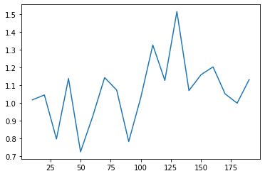
The model was trained for 20 epochs on Google Colab for an hour; the graph of the loss over time is shown below.

Testing the Model
Now let’s test our signature verification system on the test data set:
-
Load the test data set using the DataLoader class from PyTorch.
-
Pass the image pairs and the labels.
-
Find the Euclidean distance between the images.
-
Print the output based on the Euclidean distance.
# Load the test data set
test_dataset = SiameseDataset(training_csv=testing_csv,training_dir=testing_dir,
                                        transform=transforms.Compose([transforms.Resize((105,105)),
                                                                      transforms.ToTensor()
                                                                      ])
                                      )

test_dataloader = DataLoader(test_dataset,num_workers=6,batch_size=1,shuffle=True)
#test the network
count=0
for i, data in enumerate(test_dataloader,0):
  x0, x1 , label = data
  concat = torch.cat((x0,x1),0)
  output1,output2 = model(x0.to(device),x1.to(device))

  eucledian_distance = F.pairwise_distance(output1, output2)

  if label==torch.FloatTensor([[0]]):
    label="Original Pair Of Signature"
  else:
    label="Forged Pair Of Signature"

  imshow(torchvision.utils.make_grid(concat))
  print("Predicted Eucledian Distance:-",eucledian_distance.item())
  print("Actual Label:-",label)
  count=count+1
  if count ==10:
    break
The predictions are as follows:

In this article, we discussed how Siamese networks are different from normal deep learning networks and implemented a signature verification system. You can find the entire code here.
Frequently Asked Questions
What is a Siamese neural network?
A Siamese neural network (SNN) is a type of neural network architecture that consists of two or more identical sub-networks with shared weights and parameters, designed to learn similarity between inputs. SNNs are commonly used in tasks like facial recognition and signature verification where labeled data is limited.
How is a Siamese network different from a regular neural network?
Unlike traditional neural network classifiers, Siamese neural networks learn a similarity function to compare distance-based similarity between inputs and don’t require retraining when adding new classes.


