Python Profiling Tools: A Tutorial

Profiling is a software engineering task in which software bottlenecks are analyzed programmatically. This process includes analyzing memory usage, the number of function calls and the runtime of those calls. Such analysis is important because it provides a rigorous way to detect parts of a software program that may be slow or resource inefficient, ultimately allowing for the optimization of software programs. 

Profiling has use cases across almost every type of software program, including those used for data science and machine learning tasks. This includes extraction, transformation and loading (ETL) and machine learning model development. You can use the Pandas library in Python to conduct profiling on ETL, including profiling Pandas operations like reading in data, merging data frames, performing groupby operations, typecasting and missing value imputation. 

Identifying bottlenecks in machine learning software is an important part of our work as data scientists. For instance, consider a Python script that reads in data and performs several operations on it for model training and prediction. Suppose the steps in the machine learning pipeline are reading in data, performing a groupby, splitting the data for training and testing, fitting three types of machine models, making predictions for each model type on the test data, and evaluating model performance. For the first deployed version, the runtime might be a few minutes. 

After a data refresh, however, imagine that the script’s runtime increases to several hours. How do we know which step in the ML pipeline is causing the problem? Software profiling allows us to detect which part of the code is responsible so we can fix it. 

Another example relates to memory. Consider the memory usage of the first version of a deployed machine learning pipeline. This script may run for an hour each month and use 100 GB of memory. In the future, an updated version of the model, trained on a larger data set, may run for five hours each month and require 500 GB of memory. This increase in resource usage is to be expected with an increase in data set size. Detecting such an increase may help data scientists and machine learning engineers decide if they would like to optimize the memory usage of the code in some way. Optimization can help prevent companies from wasting money on unnecessary memory resources. 

Python provides useful tools for profiling software in terms of runtime and memory. One of the most basic and widely used is the timeit method, which offers an easy way to measure the execution times of software programs. The Python memory_profile module allows you to measure the memory usage of lines of code in your Python script. You can easily implement both of these methods with just a few lines of code.

We will work with the credit card fraud data set and build a machine learning model that predicts whether or not a transaction is fraudulent. We will construct a simple machine learning pipeline and use Python profiling tools to measure runtime and memory usage. This data has an Open Database License and is free to share, modify and use. 

More From Sadrach PierreHow to Find Outliers (With Examples)

Preparing Data 

To start, let’s import the Pandas library and read our data into a Pandas data frame:

df = pd.read_csv("creditcard.csv")

Next, let’s relax the display limits for columns and rows using the Pandas method set_option():

pd.set_option('display.max_columns', None)
pd.set_option('display.max_rows', None)

Next, let’s display the first five rows of data using the head() method:

print(df.head())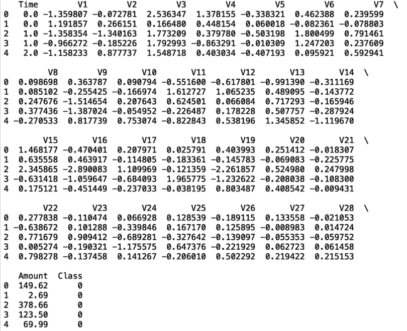

Next, to get an idea of how big this data set is, we can use the len method to see how many rows there are:

print("Number of rows: ", len(df))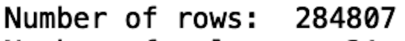

And we can do something similar for counting the number of columns. We can assess the columns attribute from our Pandas data frame object and use the len() method to count the number of columns:

print("Number of columns: ", len(df.columns))

We can see that this data set is relatively large: 284,807 rows and 31 columns. Further, it takes up 150 MB of space. To demonstrate the benefits of profiling in Python, we’ll start with a small subsample of this data on which we’ll perform ETL and train a classification model. 

Let’s proceed by generating a small subsample data set. Let’s take a random sample of 10,000 records from our data. We will also pass a value for random_state, which will guarantee that we select the same set of records every time we run the script. We can do this using the sample() method on our Pandas data frame:

df = df.sample(10000, random_state=42)

Next, we can write the subsample of our data to a new csv file:

df.to_csv("creditcard_subsample10000.csv", index=False)

Defining Our ML Pipeline

Now we can start building out the logic for data preparation and model training. Let’s define a method that reads in our csv file, stores it in a data frame and returns it:

def read_data(filename):
    df = pd.read_csv(filename)
    return df

Next, let’s define a function that selects a subset of columns in the data. The function will take a data frame and a list of columns as inputs and return a new one with the selected columns:

def data_prep(dataframe, columns):
    df_select = dataframe[columns]
    return df_select

Next, let’s define a method that itself defines model inputs and outputs and returns these values:

def feature_engineering(dataframe, inputs, output):
    X = dataframe[inputs]
    y = dataframe[output]
    return X, y

We can then define a method used for splitting data for training and testing. First, at the top of our script, let’s import the train_test_split method from the model_selection module in Scikit-learn:

from sklearn.model_selection import train_test_split

Now we can define our method for splitting our data:

def split_data(X, y):
    X_train, X_test, y_train, y_test = train_test_split(X, y, 
random_state=42, test_size = 0.33)
    return X_train, X_test, y_train, y_test

Next, we can define a method that will fit a model of our choice to our training data. Let’s start with a simple logistic regression model. We can import the logistic regression class from the linear models module in Scikit-learn:

from sklearn.linear_models import logistic_regression

We will then define a method that takes our training data and an input that specifies the model type. The model type parameter we will use to define and train a more complex model later on:

def model_training(X_train, y_train, model_type):
    if model_type == 'Logistic Regression':
        model = logistic_regression()
        model.fit(X_train, y_train)
    return model

Next, we can define a method that take our trained model and test data as inputs and returns predictions:

def predict(model, X_test):
    y_pred = model.predict(X_test)
    return y_pred

Finally, let’s define a method that evaluates our predictions. We’ll use average precision, which is a useful performance metric for imbalance classification problems. An imbalance classification problem is one where one of the targets has significantly fewer examples than the other target(s). In this case, most of the transaction data correspond to legitimate transactions, whereas a small minority of transactions are fraudulent:

def evaluate(y_pred, y_test):
    precision = average_precision_score(y_test, y_pred)
    print("precision: ", precision)

Now we have all of the logic in place for our simple ML pipeline. Let’s execute this logic for our small subsample of data. First, let’s define a main function that we’ll use to execute our code. In this main function, we’ll read in our subsampled data:

def main():
    data = read_data('creditcard_subsample10000.csv')

Next, use the data prep method to select our columns. Let’s select V1, V2, V3, Amount and Class:

def main():
    ... # preceding code left out for clarity
    columns = ['V1', 'V2', 'V3', 'Amount', 'Class']
    df_select = data_prep(data, columns)

Let’s then define inputs and output. We will use V1, V2, V3, and Amount as inputs; the class will be the output:

def main():
    ... # preceding code left out for clarity
    inputs = ['V1', 'V2', 'V3']
    output = 'Class'
    X, y = feature_engineering(df_select, inputs, output)

We’ll split our data for training and testing:

def main():
    ... # preceding code left out for clarity
    X_train, X_test, y_train, y_test = split_data(X, y)

Fit our data:

def main():
    ... # preceding code left out for clarity
    model_type = 'Logistic Regression'
    model = model_training(X_train, y_train, model_type)

Make predictions: 

def main():
    ... # preceding code left out for clarity
    y_pred = predict(model, X_test)

And, finally, evaluate model predictions:

def main():
    ... # preceding code left out for clarity
    evaluate(y_pred, y_test)

We can then execute the main function with the following logic:

if __name__ == "__main__":
    main()

And we get the following output:

Now we can use some profiling tools to monitor memory usage and runtime. 

Let’s start by monitoring runtime. Let’s import the default_timer from the timeit module in Python:

from timeit import default_timer as timer

Profiling Runtime

Next, let’s start by seeing how long it takes to read our data into a Pandas data frame. We define start and end time variables and print the difference to see how much time has elapsed:

def main():
    #read in data
    start = timer()
    data = read_data('creditcard_subsample10000.csv')
    end = timer()
    print("Reading in data takes: ", end - start)
    ... # proceeding code left out for clarity

If we run our script, we see that it takes 0.06 seconds to read in our data:

Let’s do the same for each step in the ML pipeline. We’ll calculate runtime for each step and store the results in a dictionary:

def main():
    runtime_metrics = dict()
    #read in data
    start = timer()
    data = read_data('creditcard_subsample10000.csv')
    end = timer()
    read_time = end - start
    runtime_metrics['read_time'] = read_time
    
    #select relevant columns
    start = timer()
    columns = ['V1', 'V2', 'V3', 'Amount', 'Class']
    df_select = data_prep(data, columns)
    end = timer()
    select_time = end - start
    runtime_metrics['select_time'] = select_time
    
    
    #define input and output
    start = timer()
    inputs = ['V1', 'V2', 'V3']
    output = 'Class'
    X, y = feature_engineering(df_select, inputs, output)
    end = timer()
    data_prep_time = end - start
    runtime_metrics['data_prep_time'] = data_prep_time
    
    
    #split data for training and testing
    start = timer()
    X_train, X_test, y_train, y_test = split_data(X, y)
    end = timer()
    split_time = end - start
    runtime_metrics['split_time'] = split_time
    
    
    #fit model
    start = timer()
    model_type = 'Logistic Regression'
    model = model_training(X_train, y_train, model_type)
    end = timer()
    fit_time = end - start
    runtime_metrics['fit_time'] = fit_time
    
    #make predictions
    start = timer()
    y_pred = predict(model, X_test)
    end = timer()
    pred_time = end - start
    runtime_metrics['pred_time'] = pred_time
    
    #evaluate model predictions
    start = timer()
    evaluate(y_pred, y_test)
    end = timer()
    pred_time = end - start
    runtime_metrics['pred_time'] = pred_time
    
    print(runtime_metrics)

We get the following output upon executing:

We see that reading in the data and fitting it are the most time-consuming operations. Let’s rerun this with the large data set. At the top of our main function, we change the file name to this:

data = read_data('creditcard.csv')

And now, let’s return our script:

We see that, when we use the full data set, reading the data into a data frame takes 1.6 seconds, compared to the 0.07 seconds it took for the smaller data set. Identifying that it was the step where we read in the data that led to the increase in runtime is important for resource management. Understanding bottleneck sources like these can prevent companies from wasting resources like compute time. 

Next, let’s modify our model training method such that CatBoost is a model option:

from catboost import CatBoostClassifier


def model_training(X_train, y_train, model_type):
    if model_type == 'Logistic Regression':
        model = LogisticRegression()
        model.fit(X_train, y_train)
    elif model_type == 'CatBoost':
        model = CatBoostClassifier()
        model.fit(X_train, y_train)        
    return model

Let’s rerun our script but now specifying a CatBoost model:

def main():
    ...
    #fit model
    start = timer()
    model_type = 'CatBoost'
    model = model_training(X_train, y_train, model_type)
    end = timer()
    fit_time = end - start
    runtime_metrics['fit_time'] = fit_time

We see the following results:

We see that by using a CatBoost model instead of logistic regression, we increased our runtime from ~two seconds to ~ 22 seconds, which is more than a tenfold increase in runtime because we changed one line of code. Imagine if this increase in runtime happened for a script that originally took 10 hours: Runtime would increase to over 100 hours just by switching the model type. 

Profiling Memory Usage 

Another important resource to keep track of is the memory. We can use the memory_usage module to monitor memory usage line-by-line in our code. First, let’s install the memory_usage module in terminal using pip:

pip install memory_profiler

We can then simply add @profiler before each function definition. For example:

@profile
def read_data(filename):
    df = pd.read_csv(filename)
    return df

@profile
def data_prep(dataframe, columns):
    df_select = dataframe[columns]
    return df_select

And so on.

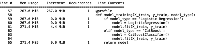
Now, let’s run our script using the logistic regression model type. Let’s look at the step where we fit the model. We see that memory usage is for fitting our logistic regression model is around 4.4 MB (line 61):

Now, let’s rerun this for CatBoost:

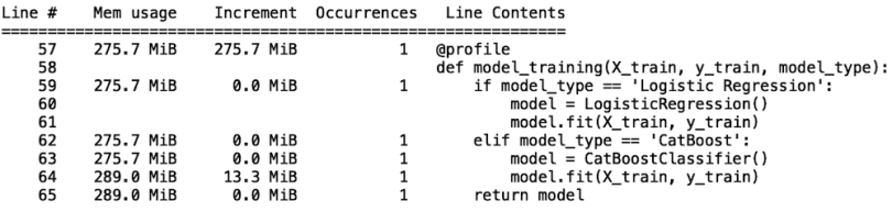
We see that memory usage for fitting our logistic regression model is 13.3 MB (line 64). This corresponds to a threefold increase in memory usage. For our simple example, this isn't a huge deal, but if a company deploys a newer version of a production and it goes from using 100 GB of memory to 300 GB, this can be significant in terms of resource cost. Further, having tools like this that can point to where the increase in memory usage is occurring is useful. 

The code used in this post is available on GitHub. 

More in Data ScienceUse Lux and Python to Automatically Create EDA Visualizations

Add Profiling to Your Toolkit

Monitoring resource usage is an important part of software, data and machine learning engineering. Understanding runtime dependencies in your scripts, regardless of the application, is important in virtually all industries that rely on software development and maintenance. In the case of a newly deployed machine learning model, an increase in runtime can have a negative impact on business. A significant increase in production runtime can result in a diminished experience for a user of an application that serves realtime machine learning predictions. 

For example, if the UX requirements are such that a user shouldn’t have to wait more than a few seconds for a prediction result and this suddenly increases to minutes, this can result in frustrated customers who may eventually seek out a better/faster tool. 

Understanding memory usage is also crucial because instances may occur in which excessive memory usage isn’t necessary. This usage can translate to thousands of dollars being wasted on memory resources that aren’t necessary. Consider our example of switching the logistic regression model for the CatBoost model. What mainly contributed  to the increased memory usage was the CatBoost package’s default parameters. These default parameters may result in unnecessary calculations being done by the package.

By understanding this dynamic, the researcher can modify the parameters of the CatBoost class. If this is done well, the researcher can retain the model accuracy while decreasing the memory requirements for fitting the model. Being able to quickly identify bottlenecks for memory and runtime using these profiling tools are essential skills for engineers and data scientists building production-ready software.