When people think of data science in general, or of specific sub-fields like natural language processing, machine learning or computer vision, they rarely consider linear algebra. We often overlook linear algebra because the contemporary tools we use to implement data science algorithms do an excellent job of hiding the underlying math that makes everything work.
Most of the time, people avoid getting into linear algebra because it’s difficult or hard to understand. Fair enough, but familiarity with linear algebra is nevertheless an essential skill for data scientists and computer engineers.
“But Sara,” you might say, “I can implement many algorithms in machine learning and data science without needing to know the math!” While that may be true to an extent, having a grasp on the fundamental mathematical principles behind the algorithms gives you a new perspective of that algorithm, hence opening up more avenues for you to explore.
In this article, I’ll discuss applications of linear algebra in three data science sub-fields. Let’s jump in!
Linear Algebra Applications for Data Scientists
- Machine learning: loss functions and recommender systems
- Natural language processing: word embedding
- Computer vision: image convolution
1. Machine Learning
Machine learning is, without a doubt, the most widely-known application of artificial intelligence (AI). Using machine learning algorithms, systems can automatically learn and improve with experience without human interference. Machine learning functions by building programs that access and analyze data (whether static or dynamic ) to find patterns and learn from. Once the program discovers relationships in the data, it can apply this knowledge to new data sets. (You can read more about how algorithms learn here.).
Linear algebra has several applications in machine learning, such as loss functions, regularization, support vector classification and many more. For our purposes, we’ll look at linear algebra in loss functions.
Loss Function
So, we know machine learning algorithms work by collecting data, analyzing it, and building a model using one of many approaches (linear regression, logistic regression, decision tree, random forest, etc.). Then, based on the results, they can predict future data queries.
But...
How can you measure the accuracy of your prediction model?
Well, by using linear algebra — loss functions, in particular. In short, loss functions are a method of evaluating the accuracy of your prediction models. Will your model perform well with new data sets? If your model is totally off, your loss function will output a higher number. Whereas, with a good model, the loss function will output a lower number.
Regression is modeling a relationship between a dependent variable, Y, and several independent variables, Xi’s. After plotting these points, we try to fit a line in space on these variables and then use this line to predict future values of Xi’s.
There are many types of loss functions, some of which are more complicated than others; however, the most commonly used two are Mean Squared Error and Mean Absolute Error.
Mean Squared Error
Mean Squared Error (MSE) is probably the most used loss error approach because it’s easy to understand, implement and generally works quite well in most regression problems. Most Python libraries like NumPy, Scikit, and TensorFlow have their own built-in implementation of the MSE functionality. Nevertheless, they all work based on the same equation:

Here, N is the number of data points in both the observed and predicted values.
Steps of calculating the MSE:
-
Calculate the difference between each pair of the observed and predicted values.
-
Take the square of the difference.
-
Add the squared differences together to find the cumulative value.
-
Calculate the average error of the cumulative sum.
Here is the Python code to calculate and plot the MSE.
#Import needed libraries
import matplotlib.pyplot as plt
#Set data
x = list(range(1,6)) #data points
y = [1,1,2,2,4]  #original values
y_bar = [0.6,1.29,1.99,2.69,3.4]  #predicted values
summation = 0
n = len(y)
for i in range(0, n):
    # finding the difference between observed and predicted value
    difference = y[i] - y_bar[i]
    squared_difference = difference**2  # taking square of the differene
    # taking a sum of all the differences
    summation = summation + squared_difference
MSE = summation/n  # get the average of all
print("The Mean Square Error is: ", MSE)
#Plot relationship
plt.scatter(x, y,  color='#06AED5')
plt.plot(x, y_bar, color='#1D3557', linewidth=2)
plt.xlabel('Data Points', fontsize=12)
plt.ylabel('Output', fontsize=12)
plt.title("MSE")
Most data scientists don’t like to use the MSE because it may not be a perfect representation of the error. However, we usually use the MSE as an intermediate step to Root Mean Squared Error (RMSE), which you can find easily by taking the square root of the MSE.
Mean Absolute Error
The Mean Absolute Error (MAE) is quite similar to the MSE; the difference is, we calculate the absolute difference between the observed data and the protected one.

The MAE cost is more robust compared to MSE. However, a disadvantage of MAE is that handling the absolute or modulus operator in mathematical equations isn’t easy. Even so, MAE is the most intuitive of all the loss function calculating methods.

Here is the Python code to calculate and plot the MAE.
#Import needed libraries
import matplotlib.pyplot as plt
#Set data
x = list(range(1,6)) #data points
y = [1,1,2,2,4]  #original values
y_bar = [0.6,1.29,1.99,2.69,3.4]  #predicted values
summation = 0
n = len(y)
for i in range(0, n):
    # finding the difference between observed and predicted value
    difference = y[i] - y_bar[i]
    abs_difference = abs(difference)  # taking square of the differene
    # taking a sum of all the differences
    summation = summation + abs_difference
MSA = summation/n  # get the average of all
print("The Mean Absolute Error is: ", MSA)
#Plot relationship
plt.scatter(x, y,  color='#06AED5')
plt.plot(x, y_bar, color='#1D3557', linewidth=2)
plt.xlabel('Data Points', fontsize=12)
plt.ylabel('Output', fontsize=12)
plt.title("MSA")Recommender Systems
Recommender systems are a class of machine learning that offer relevant suggestions to users based on pre-collected data. Recommender systems use data collected from the user’s previous interaction with the algorithm based on their preferences, demographics and other available data to predict items the current user (or a new one) might like. In doing so, companies can gain and retain customers by personalizing content to each user’s preferences.
Recommender systems functionality result from collecting two kinds of information: characteristic information and user-item interactions.
Characteristic Information
This is information about items, such as their category or price, user preferences and location.
User-Item Interactions
This includes ratings and the number of purchases (or purchases of related items).
Based on based on the desired function of the recommendation system, developers choose one of three commonly used algorithms to build it:
-
Content-based systems, which use characteristic information.
-
Collaborative filtering systems, which are based on user-item interactions.
-
Hybrid systems, which combine both types of information and aim to provide a more accurate recommendation than using only one kind of data.

To achieve optimal filtering, developers represent the information as a matrix and then use linear algebra techniques to filter out unrelated information.
2. Computer Vision
Computer vision is a field of artificial intelligence that trains computers to interpret and understand the visual world by using images, videos and deep learning models. Doing so allows algorithms to accurately identify and classify objects. In other words, algorithms learn to see visual data.
In computer vision, we use linear algebra in applications such as image recognition including some image processing techniques such as image convolution and image representation as tensors (or as we call them in linear algebra, vectors).
Image Convolution
I know what you’re thinking. “Convolution” sounds pretty...convoluted. The truth is, it’s really not! Even if you don’t think you’ve ever done computer vision before, I’m sure you’ve either done image convolution or at least seen it in action. Have you ever blurred or smoothed an image? That’s convolution!
Convolutions are one of the fundamental building-blocks in computer vision in general (and image processing in particular). To put it succinctly, convolution is an element-wise multiplication of two matrices followed by a sum. In image processing applications, a multidimensional array represents mages. An array is multi-dimensional when it has rows and columns representing the pixels of the image as well as other dimensions for the color data. For example, RGB images have a depth of three and we use them to describe any pixel’s corresponding red, green and blue color.
One way to think about image convolution is to think about the image as a big matrix and a kernel (i.e. the convolutional matrix) as a small matrix used for blurring, sharpening, edge detection or any other image processing functions. So, this kernel passes on top of the image sliding from left to right and in a top to bottom motion. While doing that, it applies some mathematical operation at each (x, y) coordinate of the image to produce a convoluted image.

Different kernels perform different types of image convolutions. Kernels are always square matrices. They are often 3x3 but you can reshape it based on the image dimensions.
To perform image convolution in Python, data scientists mostly use the OpenCV library. However, we can create arbitrary images using NumPy to practice our knowledge. Here’s a Python code to detect vertical edges in a “fake” image (NumPy array).
#Import needed libraries
import numpy as np
import matplotlib.pyplot as plt

# Create three images with different features
plain_img = np.array([np.array([100, 100]), np.array([100, 100])])
img_with_edge = np.array([np.array([100, 0]), np.array([100, 0])])

#Create a kernel to detect vertical edges (sobel, gradient edge detecting kernel)
kernel_vertical = np.array([np.array([2, -2]), np.array([2, -2])])

#Function to apply a kernel to an image
# elementwise multiplication followed by a sum
def apply_kernel(img, kernel):
return True if(np.sum(np.multiply(img, kernel))!=0) else False

#---------------------------------------------------------------------------------

# Plain Image (image with no edges)
plt.imshow(plain_img)
plt.axis('off')
plt.show()

#Printing results of applying kernal 0 if an edge is not found
if apply_kernel(plain_img,kernel_vertical):
    print("An edge has been found")
else:
    print("No edges were found")

#---------------------------------------------------------------------------------

#Image with an edge
plt.imshow(img_with_edge)
plt.axis('off')
plt.show()

#Printing results of applying kernel 0 if an edge is not found
if apply_kernel(img_with_edge,kernel_vertical):
    print("An edge has been found")
else:
    print("No edges were found")
3. Natural Language Processing
Natural Language Processing (NLP) is a branch of artificial intelligence that deals with the interaction between computers and humans using natural language — most often, English. NLP includes applications such as ChatBots, speech recognition and text analysis. I assure you, you’ve used an NLP application before. Have you ever used Grammarly or any other text grammar editors? What about digital assistants like Siri or Alexa? They are built based on the concepts of NLP.
Word Embedding
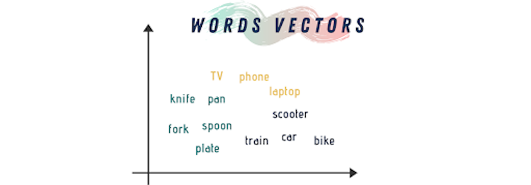
Computers can’t understand text data — not on their own anyway. That's why we perform NLP techniques on text: We need to represent the test data numerically. Here’s where algebra comes in! Word embedding is a type of word representation that allows machine learning algorithms to understand words with similar meanings.
Okay, where’s the math?
Word embeddings represent words as vectors of numbers while preserving their context in the document. These representations are obtained by training different neural networks on a large amount of text called a corpus, a language modeling learning technique. One of the most used word embedding techniques is called Word2vec.
Word2vec
Word2vec is a technique to produce word embedding for better word representation. It does that by capturing a large number of precise syntactic and semantic relationships. Word2vec learns word meanings by checking its surrounding context. Word2vec utilizes two methods:
-
Continuous bag of words: predicts the current word using context clues within a specific window.
-
Skip gram: predicts the surrounding context clues within a specific window given the current word.
Here’s a Python code that implements the Word2Vec technique using Spacy and Sklearn libraries.
#Import needed library
import spacy
from sklearn import svm
#Loading NLP dictionary from Spacy
nlp = spacy.load("en_core_web_md")

#Build a class for categories
class Category:
    BOOKS = "BOOKS"
    CANDY = "CANDY"
#Train data
train_x = ["i love the book", "this is a great book", "this tastes great", "i love the chocolate"]
train_y = [Category.BOOKS, Category.BOOKS, Category.CANDY, Category.CANDY]

#Create words vectors
docs = [nlp(text) for text in train_x]
train_x_word_vectors = [x.vector for x in docs]

#Match vectors to training data
clf_svm_wv = svm.SVC(kernel='linear')
clf_svm_wv.fit(train_x_word_vectors, train_y)

#Test new data
test_x = ["I went to the store and bought gummies", "let me check that out"]
test_docs = [nlp(text) for text in test_x]
test_x_word_vectors =  [x.vector for x in test_docs]
clf_svm_wv.predict(test_x_word_vectors)
Dimensionality Reduction
We live today in a world surrounded by massive amounts of data that needs to be processed, analyzed and stored. If we’re talking about image data, then we have a high-resolution image or video, which then translates to huge matrices of numbers. Dealing with large matrices can be a challenging task even for supercomputers, that’s why we sometimes reduce the original data to a smaller subset of features that are the most relevant to our application.
The most famous approach to reduce the dimensions of data is called singular-value decomposition (SVD). SVD is a matrix decomposition method used for reducing a matrix to its essential parts to make matrix calculations simpler. SVD is the basic concept of the latent semantic analysis (LSA) technique, which we use in topic modeling, an unsupervised ML technique that matches words to topics across various text documents. In NLP, topics are represented as clusters of related words. A topic model analyzes the various topics, their distributions in each document and the frequency of different words they contain.
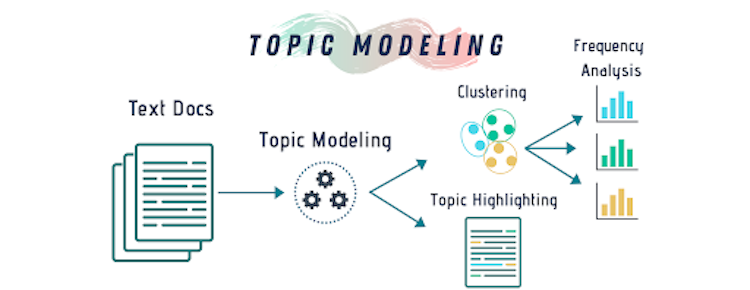
Steps of Topic Modeling
-
Create a matrix representation of a text document.
-
Use SVD to break the text matrix into three sub-matrices: document-topic matrix, topic importance diagonal matrix and topic-term matrix.
-
Reduce the dimensions of the matrices based on the importance of the topics.
We then use these smaller matrices to match words to the topic and create a distribution of words and topics.
Of course, there are many more applications of linear algebra in data science fields; we could literally talk about that for days. Linear algebra is used in all areas of computer science as well, in all kind of cybersecurity algorithms, clustering algorithms, optimization algorithms and it’s basically the only kind of math you need in quantum computing — but that’s a story for another day.