A Guide to Using ggmap in R

In R, ggmap is a package that allows users to retrieve and visualize spatial data from Google Maps, Stamen Maps or other similar map services. With it, you can create maps that display your data in a meaningful way, providing a powerful tool for data visualization and exploration.

Adding spatial and map capabilities with ggmap can be a great way to enhance your data science or analytics projects. Whether you want to showcase some examples on a map or because you have some geographical features to build algorithms, having the ability to combine data and maps is a great asset for any developer.

In this post, I’ll be taking you on a journey through the world of ggmap, exploring its features and capabilities and showing you how it can transform the way you work with spatial data. Whether you’re a data scientist, a geographic information specialist professional or simply someone with an interest in maps and spatial analysis, this post should help you to grasp the basic concepts of the ggmap package using the R programming language.

Let’s get started.

How to Install ggmap in R

To use ggmap, you first need to install the package in R. This can be done by running the following command:

install.packages("ggmap")

Once the package is installed, you can load it into your R session by running the usual library command:

library(ggmap)

The first thing we need to do is to create a map. We can do that using get_map(), a function to retrieve maps using R code.

More on RGrouping Data With R

How to Use get_map() in ggmap

This function takes a number of arguments that allow you to specify the location, type (such as street, satellite and terrain, etc.) and the source of a map. For example, the following code retrieves a street map of Lisbon, using Stamen as a source:

lisbon_map <- get_map(location ='lisbon', source="stamen")

In ggmaps, you can also use Google Maps as your source. To do that, we will need to set up a Google Maps API key, which we will cover later in the article.

When you run the code above, you will notice something odd in the output:

Google now requires an API key; see `ggmap::register_google()`

This happens because the argument location uses Google Maps to translate the location to tiles. To use get_map without relying on Google Maps, we’ll need to rely on the library osmdata:

install.packages('osmdata')
library(osmdata)

Now, we can use the function getbb, get boundary box, and feed it to the first argument of the function:

lisbon_map <- get_map( getbb('lisbon'), source="stamen")

With the code above, we’ve just downloaded our map into an R variable. By using this variable, we’ll be able to plot our downloaded map using ggplot-like features.

Plotting our Map in ggmap

Once we have retrieved the map, we can use the ggmap() function to view it. This function takes the map object that we created with get_map(), and plots it in a 2D format:

ggmap(lisbon_map)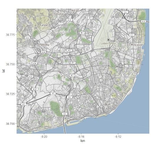

On the x-axis, we have the longitude of our map, while in the y we are able to see the latitude. We can also ask for other types of maps, by providing a maptype argument on get_map:

lisbon_watercolor <- get_map( getbb('lisbon'), maptype='watercolor', source="stamen")
ggmap(lisbon_watercolor)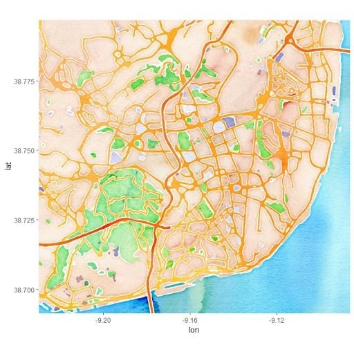

Also, you can pass coordinates to the function as arguments. However, in order to use this function, you will need to set up your Google Maps API.

Unlocking Google Maps as a source for the ggmap package will give you access to a range of useful features. With the API set up, you will be able to use the get_map function to retrieve map images based on specified coordinates, as well as unlocking new types and sizes of the map image.

Using Google Services With ggmap

Using ggmap without Google Maps will prevent you from using a bunch of different features that are very important, such as:

• Transforming coordinates into map queries.
• Accessing different types of maps such as satellite images or roadmaps.

So let’s continue to use ggmap, but this time using Google services by providing a Google Maps API key. To use it, you need to have a billing address active on Google Cloud Platform, so proceed at your own risk. I also recommend you set up billing alerts, in case Google Maps API pricing changes in the future.

To register your API key in R, you can use the register_google function:

api_secret <- '#### YOUR API KEY'

register_google(key = api_secret)

Now, you can ask for several cool things, for example, satellite maps:

lisbon_satellite <- get_map(‘Lisbon’, maptype=’satellite’, source=”google”, api_key = api_secret)

Visualizing our new map:

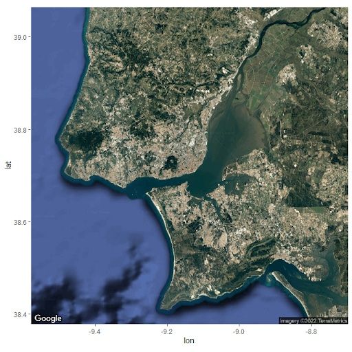
 We can also tweak the zoom parameter for extra detail on our satellite:

lisbon_satellite <- get_map('Lisbon', maptype='satellite', source="google", api_key=api_secret, zoom=15)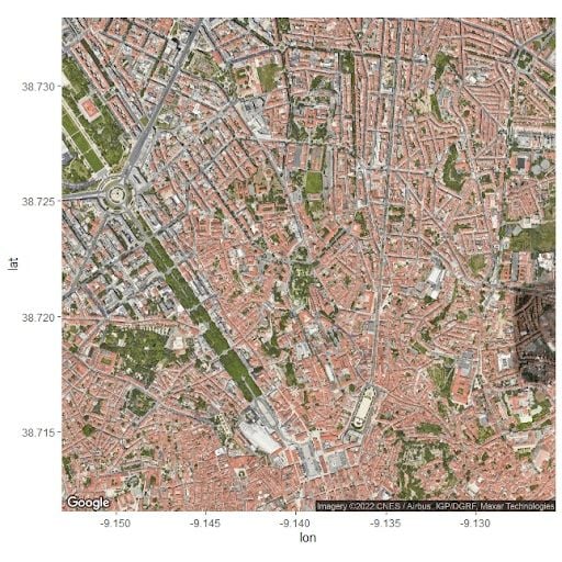

Another familiar map that we can access with google services is the famous roadmap:

lisbon_road <- get_map('Lisbon', maptype='roadmap', source="google", api_key = api_secret, zoom=15)
ggmap(lisbon_road)

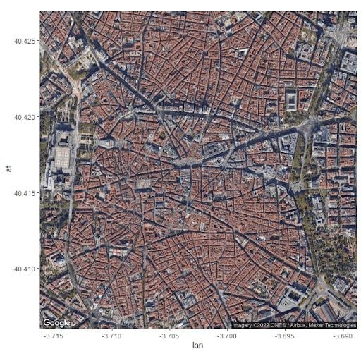
Now, we can also provide coordinates to location, instead of a named version:

madrid_sat <- get_map(location = c(-3.70256, 40.4165), maptype='satellite', source="google", api_key = api_secret, zoom=15)
ggmap(madrid_sat)

The madrid_sat map is a map centered on Madrid. We gave the Madrid coordinates to get_map by passing a vector with longitude and latitude to the location argument.

So far, we’ve seen the great features regarding map visualization using the ggmap. But, of course, these maps should be able to integrate with our R data. Next, we’ll cover the most interesting part of this post, mixing R Data with our ggmap.

Adding Data in ggmap

You can also use ggmap to overlay your own data on the map. First, we will create a sample DataFrame, and then use the geom_point() functions from the ggplot2 package to add those coordinates to the map.

Let’s create a data frame from two famous locations in Portugal, Torre de Belém and Terreiro do Paço, and then use geom_point() to add those locations to the map:

lisbon_locations <- data.frame(lat = c(38.70742536396477, 38.69171766489758),
                              lon = c(-9.136270433729706, -9.216095320576182))

We can now overlay our lisbon_locations on top of ggmap:

lisbon_map <- get_map('Lisbon', maptype='satellite', source="google", api_key = api_secret, zoom=12)

ggmap(lisbon_map) +
 geom_point(data = lisbon_locations, aes(x = lon, y = lat), color = "orange", size = 4)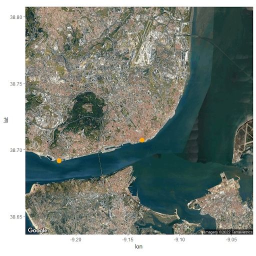

Also, we can rely on geom_segment to connect the two dots:

(
  ggmap(lisbon_map) 
  +
  geom_point(data = lisbon_locations, aes(x = lon, y = lat), color = "orange", size = 4)
  +
  geom_segment(
    data = lisbon_locations,
    aes(x = lon[1], y = lat[1], xend = lon[2], yend = lat[2]),
    color = "orange",
    size = 2
  )
)

With just a few lines of code, we can easily retrieve and visualize spatial data from Google Maps and add our coordinates to it, providing a valuable tool for data exploration and visualization.Finally, we can also work with shapefiles and other complex coordinate data in our plot. For example, I’ll add the Lisbon Cycling Roads to the map above by reading a shapefile and plotting it using geom_polygon:

library(geojsonio)
cycling_df <- geojson_read("Ciclovias.geojson",  what = "sp")

ggmap(lisbon_map) +
 geom_polygon(data = cycling_df, aes(x = long, y = lat, group = group), fill = "red")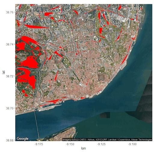

Although not perfect, the map above is a pretty detailed visualization of Lisbon’s cycling areas, with just a few errors. We’ve built this map by:

• Loading geo data using a geojson file.
• Adding a geom_polygon with red color to our ggmap.

More on RThe Ultimate Guide to Logical Operators in R

Advantages of ggmap in R

The ggmap package in R provides a useful tool for working with spatial data and creating maps for data visualization and exploration. It allows users to retrieve and visualize maps from various sources, such as Google Maps, Stamen Maps, and others, and provides options for customizing the map type, location and size.

Additionally, setting up a Google Maps API can unlock additional features, such as the ability to transform coordinates into map queries and access different types of maps. Overall, incorporating spatial and map capabilities into data science projects can greatly enhance your data storytelling skills and provide valuable insights.