A Guide to Metaheuristic Optimization for Machine Learning Models in Python

Mathematical optimization is the process of finding the best set of inputs that maximizes (or minimizes) the output of a function. In the field of optimization, the function being optimized is called the objective function. A wide range of out-of-the-box tools exists for solving optimization problems, though these only work with well-behaved functions, also called convex functions. Well-behaved functions contain a single optimum, whether it is a maximum or a minimum value. Here, we can think of a function as a surface with a single valley (minimum) and/or hill (maximum). Non-convex functions, therefore, are like surfaces with multiple valleys and hills. 

The optimization of convex functions, also called convex optimization, works well for simple tasks such as portfolio optimization, flight scheduling, developing optimal advertising and in machine learning. In the context of machine learning, convex optimization works when training several kinds of machine learning models, including linear regression, logistic regression and support vector machines. 

A limitation of convex optimization is it assumes that the objective function is guaranteed to have one valley and/or hill. In technical terms, convex functions are guaranteed to have what is called a global maximum or minimum. In practice, however, many objective functions do not have this characteristic, which makes them non-convex functions, because many objective functions that are used in real-life applications are very complex and contain many hills and valleys. When objective functions contain many hills and valleys, finding the lowest valley or the highest hill is typically difficult. 

Metaheuristic optimization, then, is the best approach to optimizing such non-convex functions. These algorithms are the best choice because they make no assumptions about how many hills and valleys the function contains. Although this approach aids in finding minimum and maximum values, these correspond to what are called local maxima (near a high hill) and minima (near a low valley). When using metaheuristic optimization to optimize non-convex functions, therefore, remember that these algorithms do not guarantee finding a global maximum (the highest hill) or minimum (lowest valley) because when optimizing non-convex functions, with many hills and valleys, finding the lowest valley or the highest hill is usually not computationally feasible. 

Despite this, metaheuristic optimization is often the only recourse for real life applications because convex optimization makes the strong assumption of a single hill and/or valley being present in the function. These algorithms often provide solutions that are near a low enough valley or high enough hill. 

This process is important for optimizing the output of a machine learning model. For example, if you build a model that predicts cement strength for a cement manufacturer, you can use metaheuristic optimization to find the optimal input values that maximize strength. A model like this takes input values corresponding to ingredient quantities in the cement mixture. The optimizer would then be able to find the quantities for each ingredient that maximizes strength.  

Python offers a wide variety of metaheuristic optimization methods. Differential evolution is a commonly used one. It works by providing a series of candidate optimal solutions and iteratively improving these solutions by moving the candidate solutions around in the search space. Maxlipo is another method that is similar to differential evolution with an additional assumption that the function is continuous, which means it has no breaks or jumps. Maxlipo is an improvement on differential evolution since it is able to find optimal values with significantly fewer function calls. This means the algorithm runs faster while still being able to find near-optimal values. Both differential evolution and Maxlipo are variants of the genetic algorithm, which works by repeatedly modifying candidate solutions until finding a near-optimal solution. 

Both of these metaheuristic optimization algorithms have easy-to-use libraries available in Python. Differential evolution can be implemented using the Python scientific computing library Scipy and Maxlipo using the Python wrapped C++ library dlib.

Here, we will build a simple machine learning model used to predict concrete strength. We will then build an optimizer that searches for the attribute values that maximize strength. We will be working with the concrete strength regression data set. 

More From Sadrach PierreA Guide to Loss Functions for Deep Learning Classification in Python

Reading in Data

Let’s start by importing the Pandas library and reading the data into a Pandas data frame:

Import pandas as pd 

df = pd.read_csv("Concrete_Data_Yeh.csv")

Next, let’s display the first five rows of data:

print(df.head())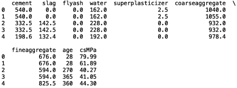

We see that the data contains columns Cement, Slag, Flyash, Water, Superplasticizeer, Coarseaggregate, Fineaggregate, Age, and CsMPa. This last column  contains values corresponding to concrete strength. We will build a random forest model that uses all the preceding inputs to predict csMPa. To proceed, let’s define our input and output:

X = df[['cement', 'slag', 'flyash', 'water', 'superplasticizer',
       'coarseaggregate', 'fineaggregate', 'age']]

y = df['csMPa']

Next, let’s split our data for training and testing:

from sklearn.model_selection import train_test_split 
X_train, X_test, y_train, y_test = train_test_split(X,y, 
test_size=0.2, random_state = 42)

Next, let’s import the random forest class from the ensemble module in Scikit learn:

from sklearn.ensemble import RandomForestRegressor

Let’s store an instance of the random forest regression class in a variable called model. We will define a random forest model with 100 estimators and a max depth of 100:

model = RandomForestRegressor(n_estimators=100, max_depth=100)

Next, let’s fit our model to our training data that was returned by the train/test split method:

model.fit(X_train, y_train)

We can then make predictions on the test set and store the predictions in a variable called y_pred:

y_pred = model.predict(X_test)

Next, let’s evaluate the performance of our regression model. We can use root mean squared error (RMSE) to evaluate how well our model performed:

from sklearn.metrics import mean_squared_error
import numpy as np 

rmse = np.sqrt(mean_squared_error(y_test, y_pred))

print("RMSE: ", rmse)

We see that our random forest model gives decent performance. We can also visualize performance using an actual versus predicted plot. Good performance is indicated by a linear relationship between actual and predicted values:

import matplotlib.pyplot as plt

plt.scatter(y_test, y_pred)
plt.title("Actual vs. Predicted")
plt.xlabel("Actual")
plt.ylabel("Predicted")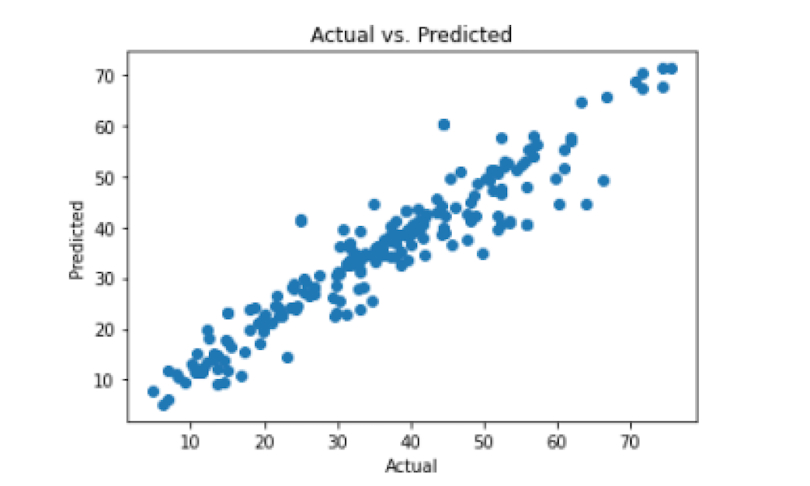

We see that we indeed have a linear relationship and our RMSE is low, so we can be satisfied with the performance of our model. 

Now that we are satisfied with our model, we can define a new model object, which we will train on the full data set:

model_full= RandomForestRegressor(n_estimators=100, max_depth=100, 
random_state =42)
model_full.fit(X, y)

The model_full object has a predict method that will serve as the function we will optimize, also called the objective function. 

The goal of our optimization task is to find the values for each of the inputsthat optimize the cement strength. 

Differential Evolution

Let’s import the differential evolution class from the optimize module in Scipy:

from scipy.optimize import differential_evolution

Next, let's define our objective function. It will take an array of inputs corresponding to the model inputs and return a prediction for each set:

def obj_fun(X):
    X = [X]
    results = model_full.predict(X)
    obj_fun.counter += 1
    print(obj_fun.counter)
    return -results

We will also print the number of function calls with each step. This will help to compare runtime performance between optimizers. Ideally, we want an optimizer that finds the maximum value the quickest, which usually translates to fewer function calls.

Next, we need to define the upper and lower bounds for each of the inputs. Let’s use the maximum and minimum values available in the data for each input:

boundaries = [(df['cement'].min(), df['cement'].max()), 
(df['slag'].min(), df['slag'].max()), (df['flyash'].min(), 
df['flyash'].max()), (df['water'].min(), df['water'].max()), 
(df['superplasticizer'].min(), df['superplasticizer'].max()),
(df['coarseaggregate'].min(), df['coarseaggregate'].max()), 
(df['fineaggregate'].min(), df['fineaggregate'].max()), 
(df['age'].min(), df['age'].max())]

Next, let’s pass our objective function and boundaries into the differential evolution optimizer:

if __name__ == '__main__':
    opt_results = differential_evolution(obj_fun, boundaries)

We can then print the optimal input and the value of the output:

if __name__ == '__main__':
    
    
    opt_results = differential_evolution(obj_fun, boundaries)
    
        
    print('cement:', opt_results.x[0])
    print('slag:', opt_results.x[1])
    print('flyash:', opt_results.x[2])
    print('water:', opt_results.x[3])
    print('superplasticizer:', opt_results.x[4])
    print('coarseaggregate:', opt_results.x[5])
    print('fineaggregate:', opt_results.x[6])
    print('age:', opt_results.x[7])
    
    print("Max Strength: ", -opt_results.fun)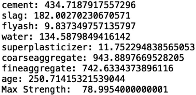

We see that the differential evolution optimizer found an optimal value of 79 after 5500 function calls. This performance is pretty poor given that it requires a large number of function calls, which makes the algorithm run very slowly. Further, the required number of function calls can’t be specified by the researcher and may actually vary between runs. This creates unpredictable runtimes for optimization. 

Maxlipo Optimizer

Maxlipo is a better alternative as it is able to find near-optimal values with fewer function calls. Further, user can specify the function calls, which resolves the issue of unpredictable runtimes. 

So, let’s build our Maxlipo optimizer. We will import the method from the dlib library in Python:

import dlib

Next, let’s define the upper and lower bounds and number of function calls:

lbounds = [df['cement'].min(), df['slag'].min(), df['flyash'].min(), 
df['water'].min(), df['superplasticizer'].min(), 
df['coarseaggregate'].min(), 
           df['fineaggregate'].min(), df['age'].min()]
ubounds = [df['cement'].max(), df['slag'].max(), df['flyash'].max(), 
df['water'].max(), df['superplasticizer'].max(), 
df['coarseaggregate'].max(), 
           df['fineaggregate'].max(), df['age'].max()]
max_fun_calls = 1000

Since the objective function needs to take a slightly different form, let’s redefine it:

def maxlip_obj_fun(X1, X2, X3, X4, X5, X6, X7, X8):
    X = [[X1, X2, X3, X4, X5, X6, X7, X8]]
    results = model_full.predict(X)
    return results

Next, we pass the boundaries, objective function and the maximum number of function calls into our optimizer:

sol, obj_val = dlib.find_max_global(maxlip_obj_fun, lbounds, ubounds, 
max_fun_calls)

Now, we can print our results from our Maxlipo optimizer:

print("MAXLIPO Results: ")
print('cement:', sol[0])
print('slag:', sol[1])
print('flyash:', sol[2])
print('water:', sol[3])
print('superplasticizer:', sol[4])
print('coarseaggregate:', sol[5])
print('fineaggregate:', sol[6])
print('age:', sol[7])


print("Max Strength: ", obj_val)

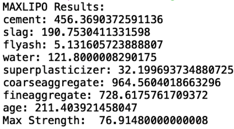
We see that the algorithm found a maximum strength of 77 with 1000 function calls. The Maxlipo algorithm found an optimal value close to what differential evolution found but with one-fifth of the function calls. Thus, the Maxlipo algorithm is five times faster than differential evolution. 

The code in this post is available on GitHub. 

Master Data Science3 Ways to Write Pythonic Conditional Statements

Optimize Away!

Optimization is an important method in computation that has a wide range of applications across industries. Given the complex nature of many machine learning models, many of the idealistic assumptions made in numerical optimization do not apply. This is why optimization methods that don’t make strong assumptions about the form of the function are important for machine learning. 

The Python libraries available for metaheuristic optimization nicely lend themselves to machine learning models. When considering optimizers, the researcher needs to understand how efficient the optimizers are in terms of runtime and function calls because it can significantly impact the time it takes to generate good results. Neglecting these factors can result in companies losing thousands of dollars to wasted computational resources. For this reason, data scientists need to have a decent understanding and familiarity with the metaheuristic optimization methods available.