Importance Sampling Explained

Importance sampling is an approximation method. It uses a mathematical transformation and is able to formulate the problem in a different way. 

In this post, we are going to:

1. Learn the basics of importance sampling
2. Get a deeper understanding by implementing the process.
3. Compare results from different sampling distributions.

What Is Importance Sampling?

Importance sampling is an approximation method. Let’s say you are trying to calculate an expectation of the function f(x), where x ~ p(x), subjected to some distribution. We have the following estimation of E(f(x)):

The Monte Carlo sampling method involves simply sampling x from the distribution p(x) and taking the average of all samples to get an estimation of the expectation. But here comes the problem: What if p(x) is very hard to sample from? Are we able to estimate the expectation based on a known and easily sampled distribution?

The answer is yes. And it comes from a simple transformation of the formula:

Where x is sampled from distribution q(x), and q(x) should not be 0. This way you’re able to estimate the expectation by sampling from another distribution q(x). And p(x)/q(x) is called as the sampling ratio or sampling weight, which acts as a correction weight to offset the probability of sampling from a different distribution.

Another thing we need to talk about the variance of estimation:

Where in this case, X is f(x)p(x)/q(x). If p(x)/q(x) is large, this will result in large variance, which we hope to avoid. On the other hand, it is also possible to select a proper q(x) that results in even smaller variance. Let’s get into an example.

More on Data ScienceLikelihood vs. Probability: What’s the Difference?

Importance Sampling Example

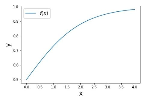
First, let’s define function f(x) and sample distribution:

def f_x(x):
    return 1/(1 + np.exp(-x))

The curve of f(x) looks like:

Now, let’s define the distribution of p(x) and q(x):

def distribution(mu=0, sigma=1):
    # return probability given a value
    distribution = stats.norm(mu, sigma)
    return distribution
    
# pre-setting
n = 1000

mu_target = 3.5
sigma_target = 1
mu_appro = 3
sigma_appro = 1

p_x = distribution(mu_target, sigma_target)
q_x = distribution(mu_appro, sigma_appro)

For simplicity, both p(x) and q(x) are normal distributions, you can try to define some p(x) that is very hard to sample from. For our first demonstration, let’s set two distributions close to each other with similar mean (3 and 3.5) and same sigma 1:

Now, we are able to compute the true value sampled from distribution p(x):

s = 0
for i in range(n):
    # draw a sample
    x_i = np.random.normal(mu_target, sigma_target)
    s += f_x(x_i)
print("simulate value", s/n)

Where we get an estimation of 0.954. Now, let’s sample from q(x) and see how it performs:

value_list = []
for i in range(n):
    # sample from different distribution
    x_i = np.random.normal(mu_appro, sigma_appro)
    value = f_x(x_i)*(p_x.pdf(x_i) / q_x.pdf(x_i))
    
    value_list.append(value)

Notice that here x_i is sampled from approximate distribution q(x), and we get an estimation of 0.949 and variance 0.304. See that we are able to get the estimate by sampling from a different distribution.

More on Data ScienceFeature Engineering Explained

Comparison

The distribution q(x) might be too similar to p(x) that you probably doubt the ability of importance sampling. So, let’s try another distribution:

# pre-setting
n = 5000

mu_target = 3.5
sigma_target = 1
mu_appro = 1
sigma_appro = 1

p_x = distribution(mu_target, sigma_target)
q_x = distribution(mu_appro, sigma_appro)

With histogram:

Here, we set n to 5000. When distribution is dissimilar, we need more samples to approximate the value. This time we get an estimation of value 0.995, but variance 83.36.

The reason comes from p(x)/q(x). Two distributions that are too different from each other could result in a huge difference of this value, thus increasing the variance. The rule of thumb is to define q(x) where p(x)|f(x)| is large.