
What Is the Central Limit Theorem?
Central limit theorem (CLT) is commonly defined as a statistical theory that given a sufficiently large sample size from a population with a finite level of variance, the mean of all samples from the same population will be approximately equal to the mean of the population.
In other words, the central limit theorem is exactly what the shape of the distribution of means will be when we draw repeated samples from a given population. Specifically, as the sample sizes get larger, the distribution of means calculated from repeated sampling will approach normality.
Central Limit Theorem Definition
Central limit theorem (CLT) is a statistical theory given that as sample sizes get larger, the mean of all samples will be approximately equal to the mean of the population, and the distribution of means will approach normality.
Let’s take a closer look at how CLT works to gain a better understanding.
Components of the Central Limit Theorem
As the sample size increases, the sampling distribution of the mean, X-bar, can be approximated by a normal distribution with mean µ and standard deviation σ/√n where:
- µ is the population mean
- σ is the population standard deviation
- n is the sample size
In other words, if we repeatedly take independent, random samples of size n from any population, then when n is large the distribution of the sample means will approach a normal distribution.
The central limit theorem states that when an infinite number of successive random samples are taken from a population, the sampling distribution of the means of those samples will become approximately normally distributed with mean μ and standard deviation σ/√ N as the sample size (N) becomes larger, irrespective of the shape of the population distribution.
How to Use the Central Limit Theorem
Suppose we draw a random sample of size n (x1, x2, x3, … xn — 1, xn) from a population random variable that is distributed with mean µ and standard deviation σ.
Do this repeatedly, drawing many samples from the population, and then calculate the x̄ of each sample.
We will treat the x̄ values as another distribution, which we will call the sampling distribution of the mean (x̄).
Given a distribution with a mean μ and variance σ2, the sampling distribution of the mean approaches a normal distribution with a mean (μ) and a variance σ2/n as n, the sample size, increases and the amazing and very interesting intuitive thing about the central limit theorem is that no matter what the shape of the original (parent) distribution, the sampling distribution of the mean approaches a normal distribution.
A normal distribution is approached very quickly as n increases (note that n is the sample size for each mean and not the number of samples).
Remember, in a sampling distribution of the mean the number of samples is assumed to be infinite.
To wrap up, there are three different components of the central limit theorem:
- Successive sampling from a population
- Increasing sample size
- Population distribution
Central Limit Theorem Formula and Example
In the image below are shown the resulting frequency distributions, each based on 500 means. For n = 4, 4 scores were sampled from a uniform distribution 500 times and the mean computed each time. The same method was followed with means of 7 scores for n = 7 and 10 scores for n = 10.
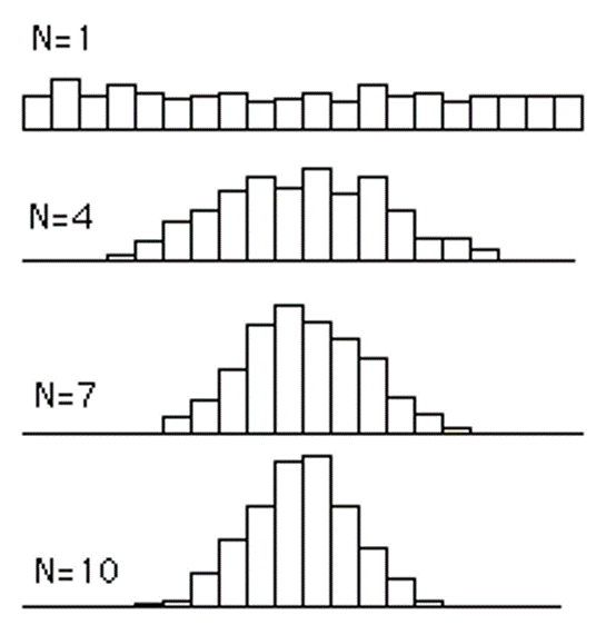
When n increases, the distributions becomes more and more normal and the spread of the distributions decreases.
Let’s look at another example using a dice.
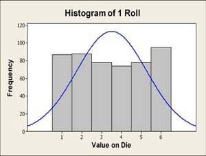
Dice are ideal for illustrating the central limit theorem. If you roll a six-sided die, the probability of rolling a one is 1/6, a two is 1/6, a three is also 1/6, etc. The probability of the die landing on any one side is equal to the probability of landing on any of the other five sides.
In a classroom situation, we can carry out this experiment using an actual die. To get an accurate representation of the population distribution, let’s roll the die 500 times. When we use a histogram to graph the data, we see that — as expected — the distribution looks fairly flat. It’s definitely not a normal distribution (figure below).
Let’s take more samples and see what happens to the histogram of the averages of those samples.
This time we will roll the dice twice, and repeat this process 500 times then compute the average of each pair (figure below).
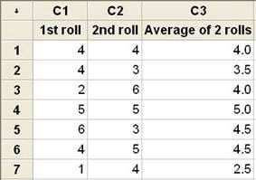
A histogram of these averages shows the shape of their distribution (figure below). Although the blue normal curve does not accurately represent the histogram, the profile of the bars is looking more bell-shaped. Now let’s roll the dice five times and compute the average of the five rolls, again repeated 500 times. Then, let’s repeat the process of rolling the dice 10 times, then 30 times.

The histograms for each set of averages show that as the sample size, or number of rolls, increases, the distribution of the averages comes closer to resembling a normal distribution. In addition, the variation of the sample means decreases as the sample size increases.
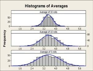
The central limit theorem states that for a large enough n, X-bar can be approximated by a normal distribution with mean µ and standard deviation σ/√n.
The population mean for a six-sided die is (1+2+3+4+5+6)/6 = 3.5 and the population standard deviation is 1.708. Thus, if the theorem holds true, the mean of the thirty averages should be about 3.5 with standard deviation 1.708/ 30 = 0.31. Using the dice we “rolled” using Minitab, the average of the thirty averages is 3.49 and the standard deviation is 0.30, which are very close to the calculated approximations.