In investing, portfolio optimization is the task of selecting assets such that the return on investment is maximized while the risk is minimized.
Portfolio Optimization Methods in Python
- Mean Variance Optimization (MVO)
- Hierarchical Risk Parity (HRP)
- Mean Conditional Value at Risk (mCVAR)
For example, an investor may be interested in selecting five stocks from a list of 20 to ensure they make the most money possible. Portfolio optimization methods, applied to private equity, can also help manage and diversify investments in private companies. More recently, with the rise in cryptocurrency, portfolio optimization techniques have been applied to investments in Bitcoin and Ethereum, among others.
In each of these cases, the task of optimizing assets involves balancing the trade-offs between risk and return, where return on a stock is the profits realized after a period of time and risk is the standard deviation in an asset's value. Many of the available methods of portfolio optimization are essentially extensions of diversification methods for assets in investing. The idea here is that having a portfolio of different types of assets is less risky than having ones that are similar.
Portfolio Optimization Methods to Know
Finding the right methods for portfolio optimization is an important part of the work done by investment banks and asset management firms.
Mean-Variance Optimization (MVO)
One of the early portfolio optimization methods is called mean-variance optimization (MVO), which was developed by Harry Markowitz and, consequently, is also called the Markowitz Method or the HM method. The method works by assuming investors are risk-averse. Specifically, it selects a set of assets that are least correlated (i.e., different from each other) and that generate the highest returns. This approach means that, given a set of portfolios with the same returns, you will select the portfolio with assets that have the least statistical relationship to one another.
For example, instead of selecting a portfolio of tech company stocks, you should pick a portfolio with stocks across disparate industries. In practice, the mean-variance optimization algorithm may select a portfolio containing assets in tech, retail, healthcare and real estate instead of a single industry like tech. Although this is a fundamental approach in modern portfolio theory, it has many limitations such as assuming that historical returns completely reflect future returns.
Hierarchical Risk Parity (HRP) and Mean Conditional Value at Risk (mCVAR)
Additional methods like hierarchical risk parity (HRP) and mean conditional value at risk (mCVAR) address some of the limitations of the mean-variance optimization method. Specifically, HRP does not require inverting of a covariance matrix, which captures how pairs of asset returns vary together. The mean-variance optimization method requires finding the inverse of the covariance matrix, however, which is not always computationally feasible.
Further, the mCVAR method does not make the assumption that mean-variance optimization makes, which happens when returns are normally distributed. Since mCVAR doesn’t assume normally distributed returns, it is not as sensitive to extreme values like mean-variance optimization. This means that if a stock has an anomalous increase in price, mCVAR will be more robust than mean-variance optimization and will be better suited for asset allocation. Conversely, mean-variance optimization may naively suggest we disproportionately invest most of our resources in an asset that has an anomalous increase in price.
The Python package PyPortfolioOpt provides a wide variety of features that make implementing all these methods straightforward. Here, we will look at how to apply these methods to construct a portfolio of stocks across industries.
Accessing Stock Price Data With Python
We will pull stock price data using the Pandas-Datareader library. You can easily install the library using pip in a terminal command line:
pip install pandas-datareaderNext, let’s import the data reading in a new Python script:
import pandas_datareader.data as web
import datetime
We should pull stocks from a few different industries, so we’ll gather price data in healthcare, tech, retail and finance. We will pull three stocks for each industry. Let’s start by pulling a few stocks in healthcare. We will pull two years of stock price data for Moderna, Pfizer and Johnson & Johnson.
First, let’s import Pandas and relax the display limits on rows and columns:
import pandas as pd
pd.set_option('display.max_columns', None)
pd.set_option('display.max_rows', None)
Next, let’s import the datetime module and define start and end dates:
start = datetime.datetime(2019,9,15)
end = datetime.datetime(2021,9,15)
Now we have everything we need to pull stock prices. Let’s get data for Moderna (MRNA):
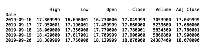
Let’s wrap this logic in a function that we can easily reuse since we will be pulling several stocks:
def get_stock(ticker):
    data = web.DataReader(f"{ticker}","yahoo",start,end)
    data[f'{ticker}'] = data["Close"]
    data = data[[f'{ticker}']]
    print(data.head())
return data 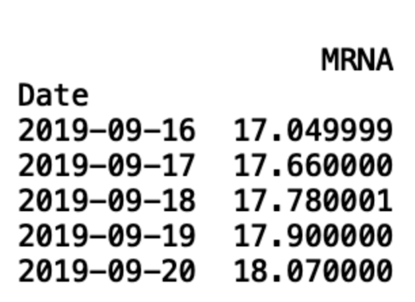
Now, let’s pull for Pfizer (PFE) and Johnson & Johnson (JNJ):
pfizer = get_stock("PFE")
jnj = get_stock("JNJ")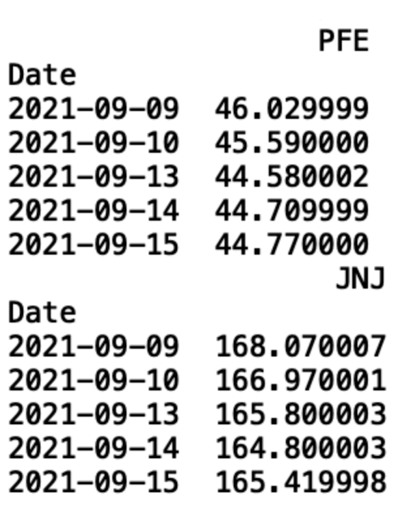
Let’s define another function that takes a list of stocks and generate a single data frame of stock prices for each stock:
from functools import reduce

def combine_stocks(tickers):
    data_frames = []
    for i in tickers:
        data_frames.append(get_stock(i))

    df_merged = reduce(lambda  left,right: pd.merge(left,right,on=['Date'], how='outer'), data_frames)
    print(df_merged.head())
    return df_merged


stocks = ["MRNA", "PFE", "JNJ"]
combine_returns(stocks)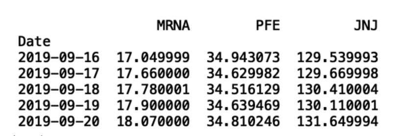
Now, let’s pull stocks for the remaining industries:
-
Healthcare: Moderna (MRNA), Pfizer (PFE), Johnson & Johnson (JNJ)
-
Tech: Google (GOOGL), Facebook (FB), Apple (AAPL)
-
Retail: Costco (COST), Walmart (WMT), Kroger Co (KR)
-
Finance: JPMorgan Chase & Co (JPM), Bank of America (BAC), HSBC Holding (HSBC)
stocks = ["MRNA", "PFE", "JNJ", "GOOGL",
          "FB", "AAPL", "COST", "WMT", "KR", "JPM",
          "BAC", "HSBC"]
portfolio = combine_stocks(stocks)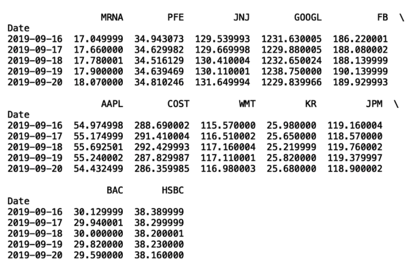
We now have a single dataframe of returns for our stocks. Let’s write this dataframe to a csv so we can easily read in the data without repeatedly having to pull it using the Pandas-Datareader.
portfolio.to_csv("portfolio.csv", index=False)Now, let’s read in our csv:
portfolio = pd.read_csv("portfolio.csv")
How to Use Mean Variance Optimization With PyPortfolioOpt
Now we are ready to implement the mean variance optimization method to construct our portfolio. Let’s start by installing the PyPortfolioOpt library:
pip install PyPortfolioOptNow, let’s calculate the covariance matrix and store the calculated returns in variables S and mu, respectively:
from pypfopt.expected_returns import mean_historical_return
from pypfopt.risk_models import CovarianceShrinkage


mu = mean_historical_return(portfolio)
S = CovarianceShrinkage(portfolio).ledoit_wolf()
Next, let’s import the EfficientFrontier module and calculate the weights. Here, we will use the max Sharpe statistic. The Sharpe ratio is the ratio between returns and risk. The lower the risk and the higher the returns, the higher the Sharpe ratio. The algorithm looks for the maximum Sharpe ratio, which translates to the portfolio with the highest return and lowest risk. Ultimately, the higher the Sharpe ratio, the better the performance of the portfolio.
from pypfopt.efficient_frontier import EfficientFrontier

ef = EfficientFrontier(mu, S)
weights = ef.max_sharpe()

cleaned_weights = ef.clean_weights()
print(dict(cleaned_weights))
We can also display portfolio performance:
ef.portfolio_performance(verbose=True)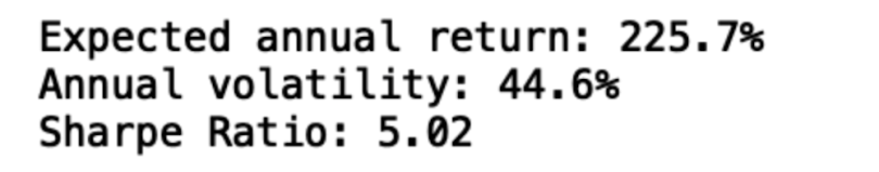
Finally, let’s convert the weights into actual allocations values (i.e., how many of each stock to buy). For our allocation, let’s consider an investment amount of $100,000:
from pypfopt.discrete_allocation import DiscreteAllocation, get_latest_prices

latest_prices = get_latest_prices(portfolio)

da = DiscreteAllocation(weights, latest_prices, total_portfolio_value=100000)

allocation, leftover = da.greedy_portfolio()
print("Discrete allocation:", allocation)
print("Funds remaining: ${:.2f}".format(leftover))
Our algorithm says we should invest in 112 shares of MRNA, 10 shares of GOOGL, 113 shares of AAPL and 114 shares of KR.
We see that our portfolio performs with an expected annual return of 225 percent. This performance is due to the rapid growth of Moderna during the pandemic. Further, the Sharpe ratio value of 5.02 indicates that the portfolio optimization algorithm performs well with our current data. Of course, this return is inflated and is not likely to hold up in the future.
Mean variance optimization doesn’t perform very well since it makes many simplifying assumptions, such as returns being normally distributed and the need for an invertible covariance matrix. Fortunately, methods like HRP and mCVAR address these limitations.
How to Use Hierarchical Risk Parity (HRP) With PyPortfolioOpt
The HRP method works by finding subclusters of similar assets based on returns and constructing a hierarchy from these clusters to generate weights for each asset.
Let’s start by importing the HRPOpt method from Pypfopt:
from pypfopt import HRPOptWe then need to calculate the returns:
returns = portfolio.pct_change().dropna()Then run the optimization algorithm to get the weights:
hrp = HRPOpt(returns)
hrp_weights = hrp.optimize()
We can now print the performance of the portfolio and the weights:
hrp.portfolio_performance(verbose=True)
print(dict(hrp_weights))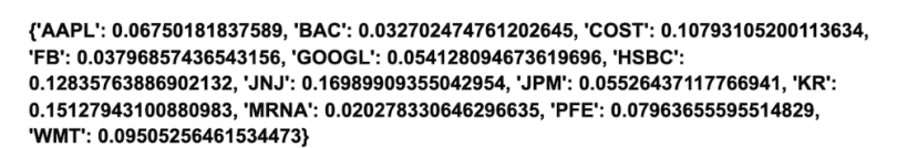
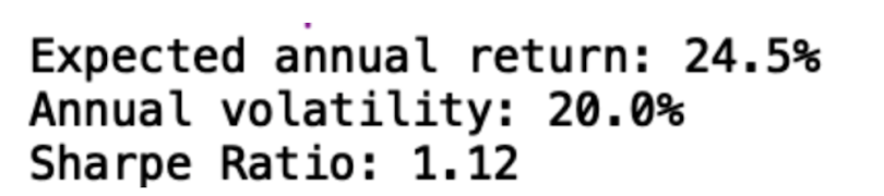
We see that we have an expected annual return of 24.5 percent, which is significantly less than the inflated 225 percent we achieved with mean variance optimization. We also see a diminished Sharpe ratio of 1.12. This result is much more reasonable and more likely to hold up in the future since HRP is not as sensitive to outliers as mean variance optimization is.
Finally, let’s calculate the discrete allocation using our weights:
da_hrp = DiscreteAllocation(hrp_weights, latest_prices, total_portfolio_value=100000)

allocation, leftover = da_hrp.greedy_portfolio()
print("Discrete allocation (HRP):", allocation)
print("Funds remaining (HRP): ${:.2f}".format(leftover))
We see that our algorithm suggests we invest heavily into Kroger (KR), HSBC, Johnson & Johnson (JNJ) and Pfizer (PFE) and not, as the previous model did, so much into Moderna (MRNA). Further, while the performance decreased, we can be more confident that this model will perform just as well when we refresh our data. This is because HRP is more robust to the anomalous increase in Moderna stock prices.
How to Use Mean Conditional Value at Risk (mCVAR) With PyPortfolioOpt
The mCVAR is another popular alternative to mean variance optimization. It works by measuring the worst-case scenarios for each asset in the portfolio, which is represented here by losing the most money. The worst-case loss for each asset is then used to calculate weights to be used for allocation for each asset.
Let’s import the EEfficicientCVAR method:
from pypfopt.efficient_frontier import EfficientCVaRCalculate the weights and get the performance:
# Convert prices to returns
returns = portfolio.pct_change().dropna()

ef_cvar = EfficientCVaR(mu, returns)
cvar_weights = ef_cvar.min_cvar()

cleaned_weights = ef_cvar.clean_weights()
print(dict(cleaned_weights))
Next, get the discrete allocation:
da_cvar = DiscreteAllocation(cvar_weights, latest_prices, total_portfolio_value=100000)

allocation, leftover = da_cvar.greedy_portfolio()
print("Discrete allocation (CVAR):", allocation)
print("Funds remaining (CVAR): ${:.2f}".format(leftover))
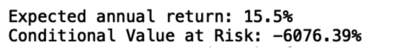
We see that this algorithm suggests we invest heavily into JP Morgan Chase (JPM) and also buy a single share each of Moderna (MRNA) and Johnson & Johnson (JNJ). Also we see that the expected return is 15.5 percent. As with HRP, this result is much more reasonable than the inflated 225 percent returns given by mean variance optimization since it is not as sensitive to the anomalous behavior of the Moderna stock price.
The code from this post is available on GitHub.
Optimize Your Portfolio
Although we only considered healthcare, tech, retail and finance, the methods we discussed can easily be modified to consider additional industries. For example, maybe you are more interested in constructing a portfolio of companies in the energy, real estate and materials industry. An example of this sort of portfolio could be made up of stocks such as Exxonmobil (XOM), DuPont (DD), and American Tower (AMT). I encourage you to play around with different sectors in constructing your portfolio.
What we discussed provides a solid foundation for those interested in portfolio optimization methods in Python. Having a knowledge of both the methods and the tools available for portfolio optimization can allow quants and data scientists to run quicker experiments for optimizing investment portfolio.
Frequently Asked Questions
What is portfolio optimization in Python?
Portfolio optimization in Python is the process of using Python tools and methods to select a mix of assets that aim to maximize return and minimize risk on an investment portfolio. In Python, portfolio optimization can be performed using packages like PyPortfolioOpt.
What methods can can be used for portfolio optimization in Python?
Methods like mean-variance optimization (MVO), hierarchical risk parity (HRP) and mean conditional value at risk (mCVAR) can be helpful for balancing portfolio return and risk when performing portfolio optimization with Python. While MVO can be skewed by outliers, HRP and mCVAR offer more robust, realistic asset allocation strategies.