Data Transformations in R

Data transformation is the process of cleaning and organizing data from one format into another. It’s one of the key aspects of work for data analysis, data science and even artificial intelligence. 

In this article, we will see how to transform data in R. R is an open-sourced programming language for statistical computing and machine learning supported by the R Foundation for Statistical Computing. It is easy to learn and comfortable to work with its widely used integrated development environment- RStudio. The R package that we will use here is tidyverse, an opinionated collection of R packages for data science.

Functions from dplyr and tidyr packages of tidyverse mostly do the work of data transformation.

 

How to Install Tidyverse for Data Transformations in R

Let’s install and load the package first.

install.packages("tidyverse")

library(tidyverse)

You will need to install the package only once, but you’ll need to load the package every time you start your environment.

More on Data ScienceWhat Is Kaggle? How to Compete in Kaggle Competitions.

 

7 Functions to Know for Transformations in R

These are the functions that we will work on in this article.

1. arrange(): This orders the observations.
2. select(): Used to select variables or columns.
3. filter(): Used to filter observations by their values.
4. gather(): This shifts observations from columns to rows.
5. spread(): This shifts variables from rows to columns.
6. group_by() and summarize(): Used to summarize data into groups.
7. mutate(): Used to create new variables from existing variables.

 

1. Arrange()

This function arranges rows by variables.

It arranges the observations in order. It takes a column name or a set of column names as arguments. For a single column name, it sorts the column’s data with other columns following that column. For multiple column names, each additional column breaks ties in the values of preceding columns.

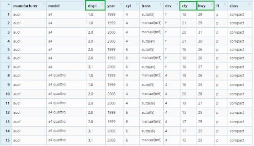
To show this, we will load the mpg data set. It has fuel economy data from 1999 to 2008 for 38 popular car models.

?mpg
data(mpg)
View(mpg)

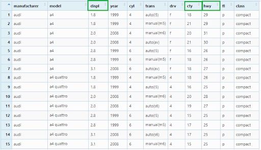
First, we will order the observations as per the “displ” column. Values of this column will be arranged in ascending order by default and other columns will follow the order of the “displ” column.

mpg_arrange1 <- mpg %>% arrange(displ)
View(mpg_arrange1)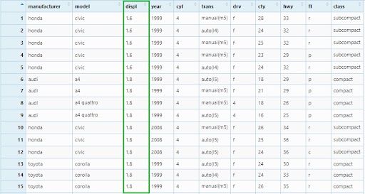

Then, we will add more two column names — cty and hwy in the arguments.

mpg_arrange2 <- mpg %>% arrange(displ, cty, hwy)
View(mpg_arrange2)

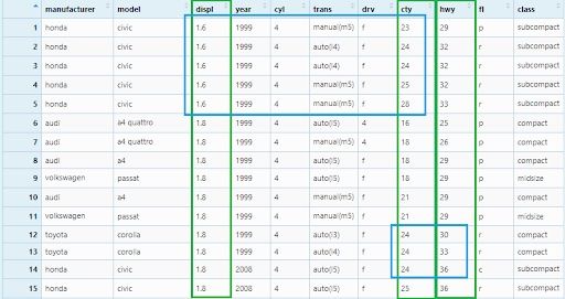
We can see the second (cty) and the third (hwy) columns are breaking the ties in the values of the first (displ) and second (cty) columns respectively.

To order the observations in descending order, we’ll use the desc()function.

mpg_arrange3 <- mpg %>% arrange(desc(displ))
View(mpg_arrange3)

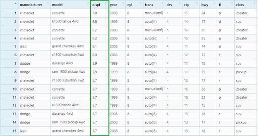
If there were any missing values, they would be sorted at the end.

 

2. Select()

Select variables by name.We will use the same mpg data set here.

?mpg
data(mpg)
View(mpg)

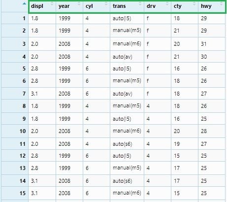
Now, we will select three columns —displ, cty and hwy to a new data frame.

mpg_select1 <- mpg %>% select(displ, cty, hwy)
View(mpg_select1)

If we want to select all columns from displ to hwy, we can write below:

mpg_select2 <- mpg %>% select(displ : hwy)
View(mpg_select2)

 

3. Filter()

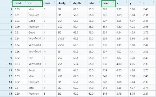
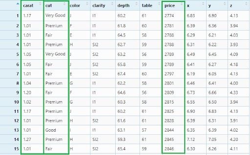
Filter observations by conditions. For this we will use the diamonds data set and see how to select observations based on conditions.

?diamonds
data(diamonds)
View(diamonds)

We can check the summary of the column’s values.

> summary(diamonds$carat)
Min. 1st Qu.  Median    Mean 3rd Qu.    Max. 
0.2000  0.4000  0.7000  0.7979  1.0400  5.0100
> summary(diamonds$price)
Min. 1st Qu.  Median    Mean 3rd Qu.    Max. 
326     950    2401    3933    5324   18823
> table(diamonds$cut)
Fair      Good Very Good   Premium     Ideal 
1610      4906     12082     13791     21551

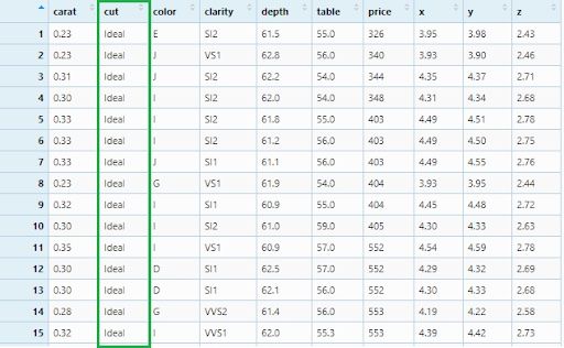
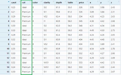
Let’s filter only the ideal cut diamonds.

diamonds_filter1 <- diamonds %>% filter(cut == 'Ideal')
View(diamonds_filter1)

Now, let’s filter ideal and premium cut diamonds.

diamonds_filter2 <- diamonds %>% 
  filter(cut == c('Ideal', 'Premium'))
View(diamonds_filter2)

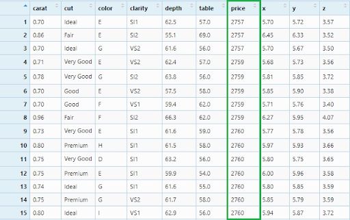
This is how we will filter diamonds with a price greater than 2500.

diamonds_filter3 <- diamonds %>% filter(price > 2500)
View(diamonds_filter3)

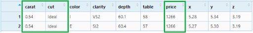
Now, we will apply our filter in three columns: Ideal cut, 0.54 carat diamonds and price equal to 1266.

diamonds_filter4 <- diamonds %>% 
  filter(cut == 'Ideal', carat == 0.54, price == 1266)
View(diamonds_filter4)

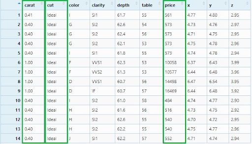
Let’s see a more complex filtering criteria: Ideal cut, between 0.4 and (&) 1.0 carat with price less than 580 or (|) greater than 10000. Appropriate logical operators will be used to express these conditions:

diamonds_filter5 <- diamonds %>% 
  filter(cut == 'Ideal' , 
         carat >= 0.4 & carat <= 1.0 , 
         price < 580 | price > 10000)
View(diamonds_filter5)

The not (!) operator needs to be used very carefully. We will need to keep in mind the De Morgan’s law while using it. This law states that !(x & y) is the same as !x | !y, and !(x | y) is the same as !x & !y.

diamonds_filter6 <- diamonds %>% 
  filter(cut != 'Ideal', 
         !(carat >= 0.4 & carat <= 1.0) , 
         !(price < 580 | price > 10000))
View(diamonds_filter6)

 

4. Gather()

Gather columns into key-value pairs. Sometimes we can have a data set where the observations are found in column names that need to be gathered under a variable with a new column name. Let’s build the data set first.

Country_Name <- c('Qatar', 'United States', 'Germany', 
                  'Canada', 'United Kingdom')
Y2009 <- c(59094, 47099, 41732, 40773, 38454)
Y2010 <- c(67403, 48466, 41785, 47450, 39080)
Y2011 <- c(82409, 49883, 46810, 52101, 41652)
gdp <- data.frame(Country_Name, Y2009, Y2010, Y2011)
View(gdp)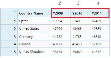

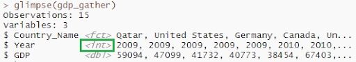
This data set can be considered as GDP data of five countries for 2009, 2010 and 2011. It is clearly seen that Y2009, Y2010 and Y2011 these column names are themselves observations and should be under a single variable or column name: ‘Year.’ We will do it using the gather() function.

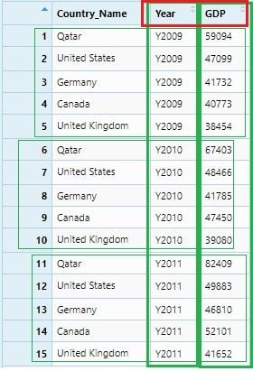
gdp_gather <- gdp %>% gather("Year", "GDP" , 2:4)
View(gdp_gather)

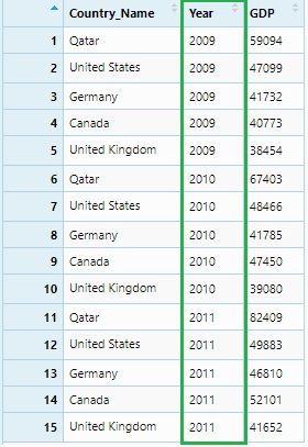
To make this data set ready for numerical analysis, we need to remove the character “Y”(or any character) from the Year values and convert it from character to integer.

gdp_gather$Year <- gsub("[a-zA-Z]", "", gdp_gather$Year)
gdp_gather$Year <- as.integer(gdp_gather$Year)
View(gdp_gather)
glimpse(gdp_gather)

 

5. Spread()

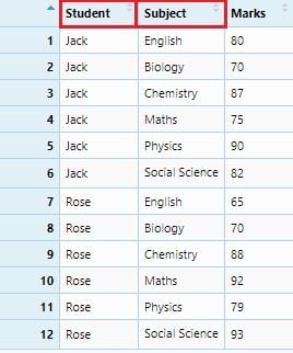
Spread a key-value pair across multiple columns. Sometimes we can see variables are distributed in observations in a dataset. In this case we need to spread it to column names. Let’s build a data set with key-values.

Student <- c('Jack', 'Jack', 'Jack', 'Jack', 'Jack', 'Jack', 
             'Rose', 'Rose', 'Rose', 'Rose', 'Rose', 'Rose')
Subject <- c('English', 'Biology', 'Chemistry', 'Maths', 'Physics', 
             'Social Science', 'English', 'Biology', 'Chemistry',
             'Maths', 'Physics', 'Social Science')
Marks <- c(80, 70, 87, 75, 90, 82, 65, 70, 88, 92, 79, 93)
reportCard <- data.frame(Student, Subject, Marks)
View(reportCard)

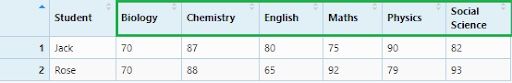
In this report card data set, if we consider the “Subject” names as variables, then it needs to spread out to the column names. We will do it through the spread() function.

reportCard_spread1 <- reportCard %>% spread(Subject, Marks)
View(reportCard_spread1)

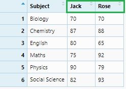
If we consider “Student” names as variables:

reportCard_spread2 <- reportCard %>% spread(Student, Marks)
View(reportCard_spread2)

 

6. Group_by() and Summarize()

Group by variables and reduce multiple values down to a single value.

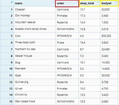
These are very useful functions that couple together to summarize values into groups. Here, we will use the mammals sleep (msleep) data set. It contains sleep and body weight data for some of the mammals.

?msleep
data(msleep)
colnames(msleep)
msleep <- msleep %>% select(name, order, sleep_total, bodywt)
View(msleep)

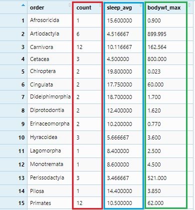
We will summarize sleep_total to its average values sleep_avg and bodywt to its maximum values bodywt_max. This summarization will be grouped as per order and the number of each order observation will be under the count column. All these will be done by group_by() and summarize() with mathematical functions: n(), mean() and max().

msleep_groupby_summarize <- msleep %>% group_by(order) %>%
  summarise(
    count = n(),
    sleep_avg = mean(sleep_total),
    bodywt_max = max(bodywt)
  )
View(msleep_groupby_summarize)

More on Data ScienceMachine Learning Basics Every Beginner Should Know

 

7. Mutate()

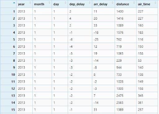
Create or transform variables. It is very common in data analysis to derive new variables from existing variables. Here we will use the flights data set. It has on-time data for all flights that departed New York City in 2013. To access this data set, we need to install and load the package nycflights13.

install.packages("nycflights13")
library(nycflights13)
?flights
data(flights)
colnames(flights)
flights <- flights %>% select(year, month, day, dep_delay, 
                              arr_delay, distance, air_time )
View(flight)

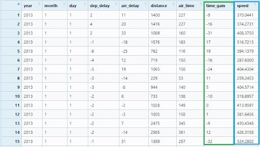
Now, we will create two new variables:time_gain by subtracting arr_delay from dep_delay and speed by dividing distance by air_timeand multiplying with 60.

flights_mutate <- flights %>% 
  mutate(time_gain = dep_delay - arr_delay ,
  speed = distance / air_time * 60)
View(flights_mutate)

I would encourage you to practice these data transformation functions with different data sets and with your own data. This could be your fist step in entering the amazing field of data science.