A Beginner’s Guide to Using Pandas for Text Data Wrangling With Python

Raw text data often comes in a form that makes analysis difficult. As such, it often requires text processing methods. Text processing is the practice of automating the generation and manipulation of text. It can be used for many data manipulation tasks including feature engineering from text, data wrangling, web scraping, search engines and much more. In this tutorial, we’ll take a look at how to use the Pandas library to perform some important data wrangling tasks.

Data wrangling is the process of gathering and transforming data to address an analytical question. It’s also often the most important and time-consuming step of the entire data science pipeline. Therefore, mastering the basic Pandas tools and skill sets is important for generating the type of clean and interpretable text data that allows for insights.

Applications of text data wrangling include removal, extraction, replacement and conversion. For example, you can remove unnecessary duplicated characters, words or phrases from text or extract important words or phrases that are key to the text’s meaning.

You can also use Pandas to replace words or phrases with more informative or useful text. Finally, Pandas can convert characters that express timestamps into datetime objects that can be used for analysis. Today, we’ll look at how to perform extraction from text as well as conversion of string values into time stamps.

More From Sadrach PierreHow Do People Feel About the COVID Vaccine?

Applying Pandas to COVID Research

An interesting application of these methods is in the context of exploring research publications relevant to a specific field or topic. Here, we’ll use the Pandas library to analyze and pull information such as titles and abstracts of research papers on the coronavirus from various journals.

Once we have this data, we can perform several analytical tasks with it, including finding the most commonly asked research questions and performing sentiment analysis on the papers’ results and conclusions. These types of analyses can then serve as a springboard for generating new research questions that have not yet been addressed.

For our purposes, we’ll be working with the COVID-19 Open Research DataSet (CORD-19), which you can find here.

To start, let’s import the Pandas library, read the file metadata.csv into a Pandas dataframe and display the first five rows of data:

import pandas as pd 

df = pd.read_csv("metadata.csv")

print(df.head())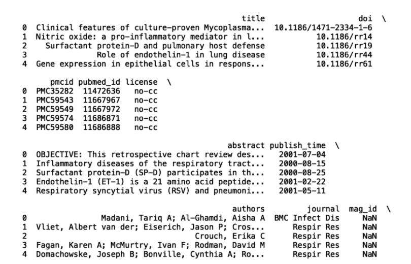

We’ll be working with the columns “title,” “abstract,” “journal” and “published_time.” Let’s filter our dataframe to only include these four columns:

df = df[['title', 'abstract', 'journal', 'published_time']].copy()

print(df.head())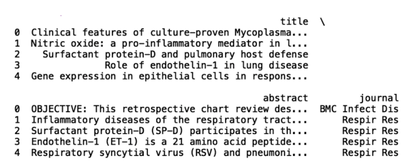

Now, let’s sample trim the data to 50,000 records and write to a new file called covid.csv:

df_new = df.sample(50000)

df_new.to_csv("covid.csv")

Now, let’s display the first five rows of data:

print(df_new.head())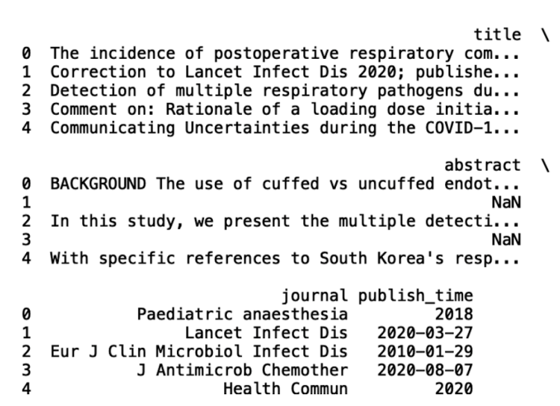

Retrieving Information From Text Using Str Accessor Method

The first operation we’ll discuss is text-based information extraction using Pandas. The first thing we can do is analyze which journals most frequently appear in the CORD-19 data. This can give insight into which ones have the most impact in the field of COVID research.

Let’s apply the counter method from the collections module to the journal column. Here, we display the 100 most frequently appearing research journals:

print(Counter(df_new['journal']).most_common(100))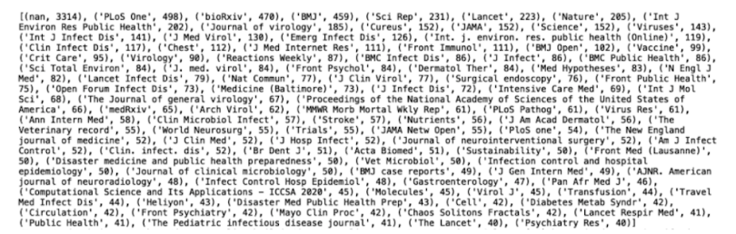

We see the most common value is actually “nan” (meaning not a number), which we can remove from our data:

df_new['journal'].dropna(inplace=True)

print(Counter(df_new['journal']).most_common(100))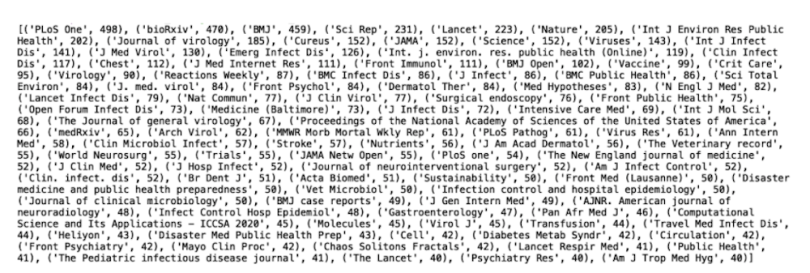

Now, we can see that the most frequently occurring journals are PLoS One, bioRxiv, BMJ, Sci Rep, Lancet and Nature.

Suppose we wanted to only look at abstracts and titles in a specific journal. We can easily filter our data on a journal name using Pandas. Let’s filter our data frame to only include records from the publication PLoS One:

df_plos = df_new[df_new['journal'] == 'PLoS One']

print(df_plos.head())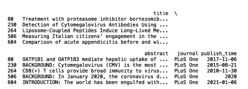

Another interesting observation is that, in our original data frame, many journals contain the words “infect” or “infections.” Suppose we are interested in journals that specialize exclusively in infectious disease research. This filtering will exclude other research areas found in the data that we may not be interested in like the gut microbiome, chemotherapy and anaesthesia, among others.

We can pull all records corresponding to journals that contain the substring “Infect Dis,” for infectious disease. We can use the contains method from the Pandas string accessor to achieve this:

df_infect = df_new[df_new['journal'].str.contains('Infect Dis', regex=False)]

print(df_infect.head())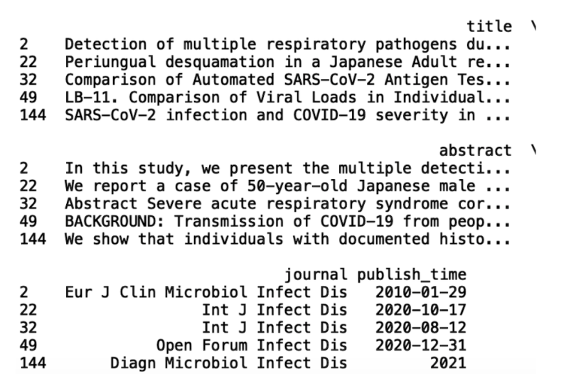

We see that our data frame, df_infect, has journal names with the substring “Infect Dis.” Within df_infect, we see two journals that contain the word “microbial.” This might pique our interest in available microbial studies. We can filter on our original data frame to only include journals with “microbial” in the name:

df_microbial = df_new[df_new['journal'].str.contains('Microbial', regex=False)].copy()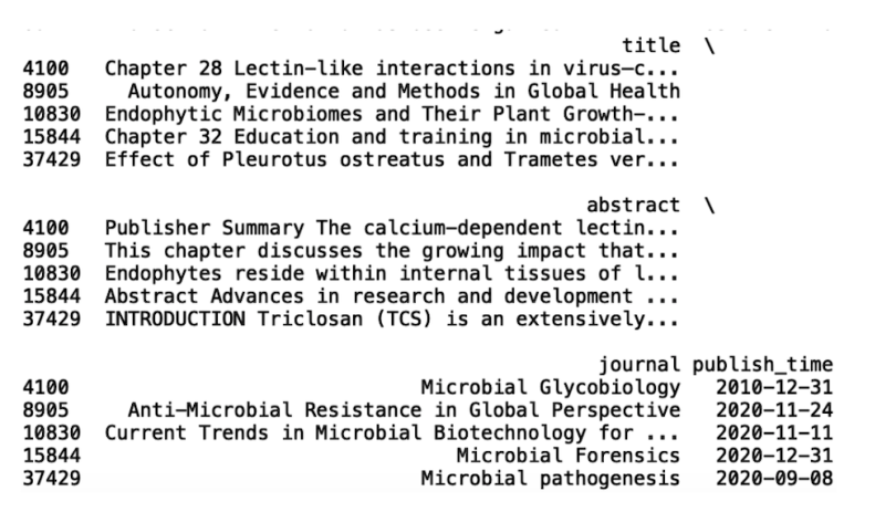

We can take our analysis in several different directions from here. Maybe we’re interested in studies that focus on the microbiome. If so, we can use the contains method further on the abstract column:

df_abstract_microbiome = df_new[df_new['abstract'].str.contains('microbiome', regex=False)].copy()

print(“Number of Microbiome Studies: “, len(df_abstract_microbiome))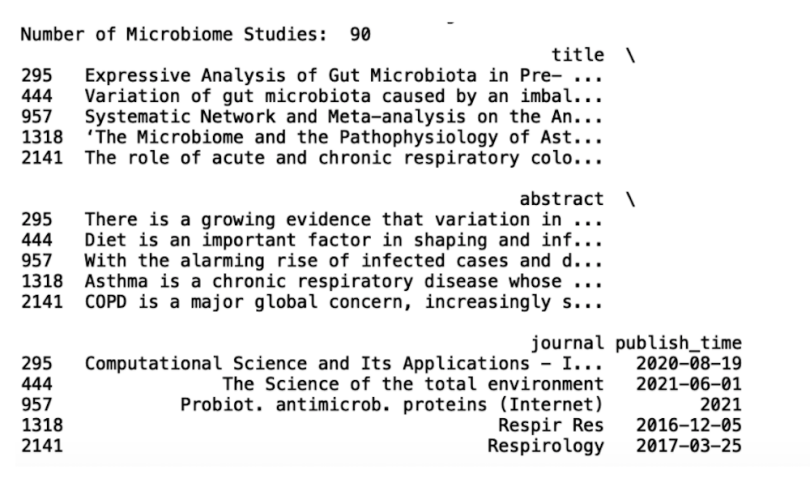

This action results in a 90-row data frame containing publications that focus on gut microbiome research. Further text analysis of the titles and abstracts allows us to address some more interesting questions:

• What kinds of questions are researchers asking about COVID-19 and gut microbiome research?
   
• Are there frequently appearing words or phrases that can give insight into the direction of research? For example, over the past few years, much research around infectious disease has turned toward understanding how gut health and diet impacts immune system function. An interesting analysis would be to see how the frequency in keywords related to the gut microbiome has changed over time.
   
• Is there a time dependent trend in frequently appearing words or phrases? Determining this can be useful for finding which questions in the space have not yet been answered. For example, if you find that, over the past five years, gut microbiome research has significantly increased, you can then filter your data to only include papers relevant to gut microbiome research. You can then perform further analysis on the abstracts to see what types of questions researchers are asking and what types of relationships they’ve discovered. This can aid in formulating novel research problems.

Here, we’ll focus on the last question. In order to do this, we need to convert the string valued time stamps into values that we can use for analysis.

Converting String Values Into Time Stamps

Converting string time values into timestamps for quantitative analysis is an important part of text data processing. If you want to analyze any time-dependent trends in your text data, this is an essential step because, in order to extract any useful information from time values (i.e., month, day or year), we need convert them from a string to a datetime value. We’ll need to do this now to answer our question from above about frequently appearing words and phrases.

First, we need to convert the publish_time”column into a Pandas datetime object. Let’s continue working with our df_abstract_microbiome data frame:

df_abstract_microbiome['publish_time'] 
= 
pd.to_datetime(df_abstract_microbiome['publish_time'], format='%Y/%m/%d')

We can create a new column that pulls the year of the publication:

df_abstract_microbiome['year'] = df_abstract_microbiome['publish_time'].dt.year

print(df_abstract_microbiome.head())

Next, let’s print the set of years:

print(set(df_abstract_microbiome['year']))

We have data from 2011 through 2021 but we’re missing the years 2012 and 2018. This absence is probably due to the filtering down of our data as well as the downsampling we performed earlier. This won’t affect our result much, as we’ll still be able to detect any time-dependent trends. Further, we can easily fix this if we want by increasing the sample size from 50,000 to a larger number.

Now, let’s use the Python library TextBlob to generate sentiment scores from the paper abstracts. Sentiment analysis is a natural language processing method that is used to understand emotion expressed in text.

A rough assumption we can make is that an abstract with negative sentiment corresponds to the larger study finding a negative relationship and vice versa.

For example, the following abstract has a positive sentiment:

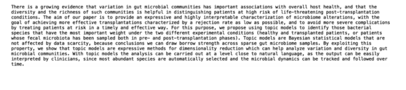
Words like “richness” and “helpful” are indicative of positive sentiment. Let’s now generate sentiment scores for our abstract column:

df_abstract_microbiome['abstract_sentiment'] = 
df_abstract_microbiome['abstract'].apply(lambda abstract: 
TextBlob(abstract).sentiment.polarity)

print(df_abstract_microbiome.head())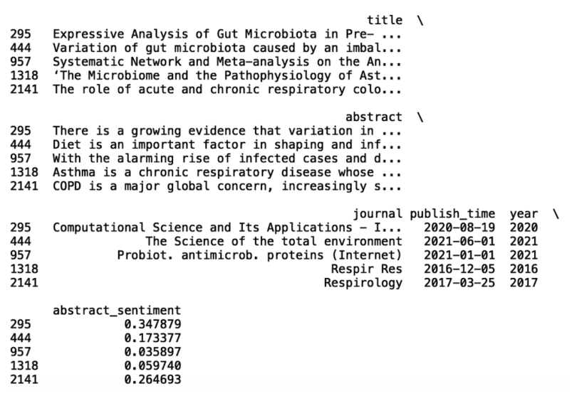

The next thing we need to do is calculate the average sentiment each year. We can achieve this using the Pandas groupby method. We can then visualize the time series data using a line plot in Matplotlib.

df_group = df_abstract_microbiome.groupby(['year'])['abstract_sentiment'].mean()

import matplotlib.pyplot as plt

import seaborn as sns

sns.set()

plt.xlabel('Year')

plt.ylabel('Sentiment')

plt.title('Research Sentiment in Gut Microbiome Studies')

plt.plot(df_group.index, df_group.values)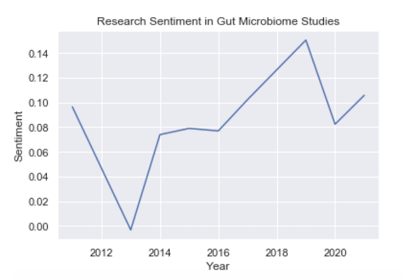

We see that there is a slight upward trend in sentiment from 2011 to 2021. This only contains 90 records, though, which isn’t much data. Let’s consider performing sentiment analysis on publications from the PLoS One journal to see if we can get some more information:

df_plos['publish_time'] = pd.to_datetime(df_plos['publish_time'], format='%Y/%m/%d')

df_plos['year'] = df_plos['publish_time'].dt.year

df_plos['abstract_sentiment'] = df_plos['abstract'].apply(lambda abstract: TextBlob(abstract).sentiment.polarity)

df_plos_group = df_pl

os.groupby(['year'])['abstract_sentiment'].mean()

import matplotlib.pyplot as plt

import seaborn as sns

sns.set()

plt.xlabel('Year')

plt.ylabel('Sentiment')

plt.title('Research Sentiment in PLoS One Publications')

plt.plot(df_plos_group.index, df_plos_group.values)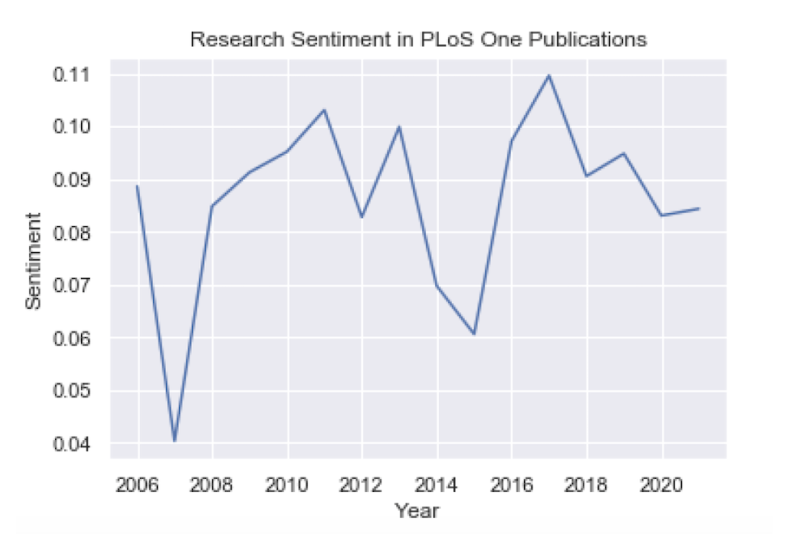

We see that for PLoS One records we have data from the years 2006 through 2021, which gives us much more to work with. In this batch, we can see a small upward trend in sentiment, but it’s fairly steady over the past 15 years.

Finally, let’s consider the publication Nature, which has the longest history of data in our sample:

df_nature = df_new[df_new['journal'] == 'Nature'].copy()

df_nature['publish_time'] = pd.to_datetime(df_nature['publish_time'], format='%Y/%m/%d')

df_nature['year'] = df_nature['publish_time'].dt.year

df_nature['abstract_sentiment'] = df_nature['abstract'].apply(lambda abstract: TextBlob(abstract).sentiment.polarity)





df_nature = df_nature.groupby(['year'])['abstract_sentiment'].mean()




import matplotlib.pyplot as plt

import seaborn as sns

sns.set()

plt.xlabel('Year')

plt.ylabel('Sentiment')

plt.title('Research Sentiment in Nature Publications')

plt.plot(df_nature.index, df_nature.values)

plt.show()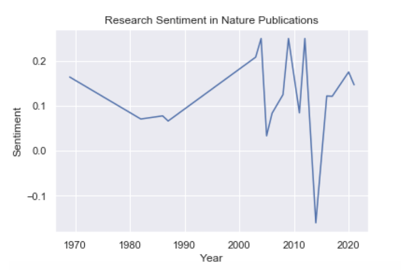

These are the three plots overlaid:

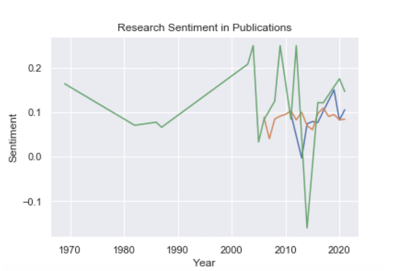
Nature seems to have more positive sentiment overall. If our assumption that the sentiment is indicative of the relationship found in a study is correct, this would mean that PLoS One may have comparatively more studies that report positive relationships.

If you are interested in accessing the code used here, it is available on GitHub.

Build Your Data Science SkillsA Comprehensive Guide to Data Visualization With Matplotlib and Seaborn

Get Started With Pandas

This analysis simply scratched the surface in terms of the types of insights you can pull from text. You can easily use these skills to take your analysis even further.

Specifically, the Pandas contains method allows you to quickly and easily search for text patterns in your data. If you’re a researcher with domain expertise, you can search for specific terms that are relevant to the kinds of questions you’d like to ask.

For example, a commonly studied protein target related to cytokine storms caused by COVID are the Janus Kinase (JAK) family proteins. You can use the contains method to search for all publications that involve JAK family proteins. Further, this type of data exploration may lead you to new problem formulations that you may not have considered before.

Sentiment analysis of research abstracts can potentially serve as a proxy for quickly qualifying findings in research studies across a large number of publications. For example, if our assumption of negative sentiment equals negative relationship in results is sound, you can use that to aid your research. Examples of negative relationships are “drug X inhibits JAK” and “drug Y inhibits sars-Cov-2.” Given the right domain expertise, Pandas and TextBlob can be used to build a high-quality research search engine to expedite the research process.

The combination of Pandas for text-based data wrangling and TextBlob for sentiment analysis is truly powerful. Oftentimes researchers are tasked with manually performing literature searches, which can be largely time consuming. These tools can aid in speeding up the process of question formulation and information retrieval for research purposes.