

Covariance vs. correlation are two distinct concepts in statistics and probability theory, but what do they actually mean in practice? More importantly, when do we use them?
Put simply: we use both of these concepts to understand relationships between data variables and values. We can quantify the relationship between variables and then use these learnings to either select, add or alter variables for predictive modeling, insight generation or even storytelling using data. Thus, both correlation and covariance have high utility in machine learning and data analysis. To learn more, let’s dive in!
Covariance vs. Correlation
Covariance reveals how two variables change together while correlation determines how closely two variables are related to each other.
- Both covariance and correlation measure the relationship and the dependency between two variables.
- Covariance indicates the direction of the linear relationship between variables.
- Correlation measures both the strength and direction of the linear relationship between two variables.
- Correlation values are standardized.
- Covariance values are not standardized.
Covariance and Correlation: What’s the Difference?
Put simply, both covariance and correlation measure the relationship and the dependency between two variables. Covariance indicates the direction of the linear relationship between variables while correlation measures both the strength and direction of the linear relationship between two variables. Correlation is a function of the covariance.
What sets these two concepts apart is the fact that correlation values are standardized whereas covariance values are not.
You can obtain the correlation coefficient of two variables by dividing the covariance of these variables by the product of the standard deviations of the same values. We’ll see what this means in practice below.
Correlation values are standardized whereas covariance values are not.
Don’t forget that standard deviation measures the absolute variability of a data set’s distribution. When you divide the covariance values by the standard deviation, it essentially scales the value down to a limited range of -1 to +1. This is precisely the range of the correlation values.
How to Calculate Covariance and Correlation
To fully understand covariance vs. correlation, we need to define the terms mathematically.
How to Calculate Covariance
The covariance of two variables (x and y) can be represented as cov(x,y). If E[x] is the expected value or mean of a sample ‘x,’ then cov(x,y) can be represented in the following way:

If we look at a single variable, say ‘y,’ cov(y,y), we can write the expression in the following way:
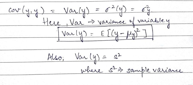
Now as we see, in the image above, ‘s²,’ or sampled variance, is basically the covariance of a variable with itself. We can also define this term in the following manner:
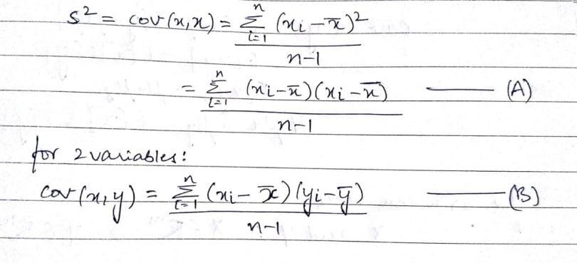
In the above formula, the numerator of the equation(A) is the sum of squared deviations. In equation(B) with two variables x and y, it’s called the sum of cross products. In the above formula, n is the number of samples in the data set. The value (n-1) indicates the degrees of freedom.
Degrees of freedom is the number of independent data points that went into calculating the estimate.
To explain degrees of freedom, let’s look at an example. In a set of three numbers, the mean is 10 and two out of three variables are five and 15. This means there’s only one possibility for the third value: 10. With any set of three numbers with the same mean, for example: 12, eight and 10 or say nine, 10 and 11, there’s only one value for any two given values in the set. Essentially, you can change the two values and the third value fixes itself. The degree of freedom here is two.
In other words, degrees of freedom is the number of independent data points that went into calculating the estimate. As we see in the example above, it is not necessarily equal to the number of items in the sample (n).
How to Calculate Correlation
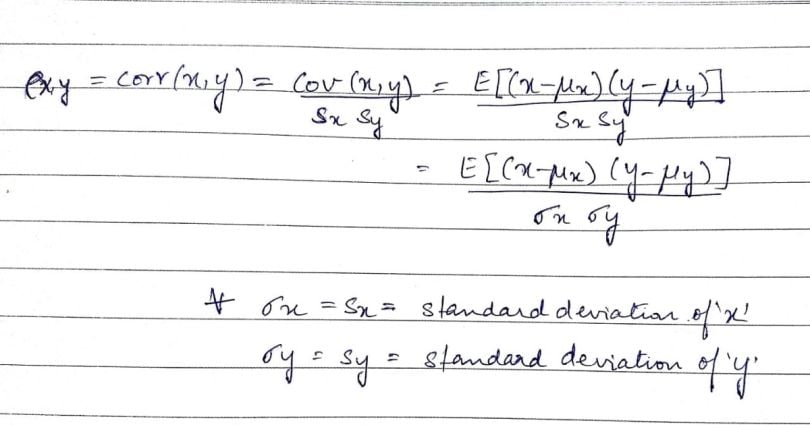
We obtain the correlation coefficient (a.k.a. the Pearson product-moment correlation coefficient, or Pearson’s correlation coefficient) by dividing the covariance of the two variables by the product of their standard deviations. Mathematically, it looks like this:

The values of the correlation coefficient can range from -1 to +1. The closer it is to +1 or -1, the more closely the two variables are related. The positive sign signifies the direction of the correlation (i.e. if one of the variables increases, the other variable is also supposed to increase).
Data Matrix Representation of Covariance and Correlation
Let’s delve a little deeper and look at the matrix representation of covariance.
For a data matrix X, we represent X in the following manner:
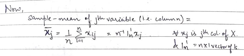
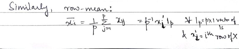
A vector ‘xj’ would basically imply a (n × 1) vector extracted from the j-th column of X where j belongs to the set (1,2,….,p). Similarly ‘xi`’ represents the (1 × p) vector from the i-th row of X. Here ‘i’ can take a value from the set (1,2,…,n).
You can also interpret X as a matrix of variables where ‘xij’ is the j-th variable (column) collected from the i-th item (row).
For ease of reference, we’ll call rows items/subjects and columns variables. Let’s look at the mean of a column of the above data matrix:
Using the above concept, let’s now define the row mean (i.e. the average of the elements present in the specified row).
Now, that we have the above metrics, it’ll be easier to define the covariance matrix (S):
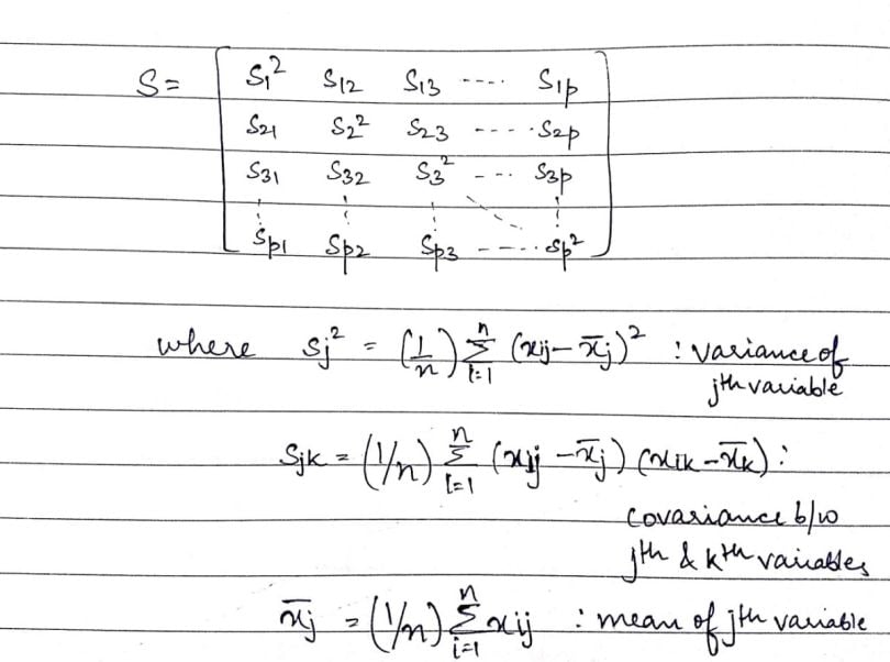
In the above matrix, we see that the dimension of the covariance matrix is p × p. This is basically a symmetrical matrix (i.e. a square matrix t equal to its transpose [S`]). The terms building the covariance matrix are called the variances of a given variable, which form the diagonal of the matrix or the covariance of two variables filling up the rest of the space. The covariance of the j-th variable with the k-th variable is equivalent to the covariance of the k-th variable with the j-th variable (i.e. ‘sjk’= ‘skj’).
We can create the covariance matrix from the data matrix in the following way:
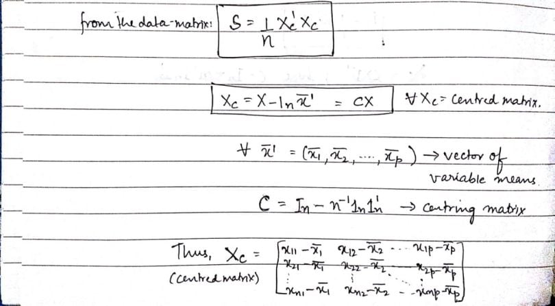
Here, ‘Xc’ is a centered matrix that has the respective column means subtracted from each element. Using that as the central component, the covariance matrix ‘S’ is the product of the transpose of ‘Xc`’ and ‘Xc’ itself, which we then divide by the number of items or rows (‘n’) in the data matrix.
Mathematics defines the value ‘s’ as the data set’s standard deviation.
Before we move forward, we should revisit the concept of sample variance or s-squared (s²). We can derive the standard deviation of a data set from this value.
Mathematics defines the value ‘s’ as the standard data set’s standard deviation. It basically indicates the degree of dispersion or spread of data around its average.
Using the same data matrix and the covariance matrix, let’s define the correlation matrix (R):

As we see here, the dimension of the correlation matrix is again p × p. Now, if we look at the individual elements of the correlation matrix, the main diagonal is comprised of one. This indicates that the correlation of an element with itself is one, or the highest value possible. The other elements, ‘rjk,’ is the Pearson’s correlation coefficient between two values: ‘xj’ and ‘xk.’ As we saw earlier, ‘xj’ denotes the j-th column of the data matrix, X.
Moving on, let’s look at how the correlation matrix can be obtained from the data matrix:
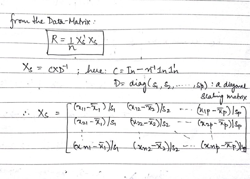
In the above definition, we call ‘Xs’ the scaled (or standardized) matrix. Here we see that the correlation matrix defined as the product of the scaled matrix’s transpose with itself, divided by ‘n’.
Upon revisiting the standard deviation definition above, it’s clear we divide every element of the standardized matrix ‘Xs’ by the respective column's standard deviation (similar to the covariance matrix above). This reinforces our understanding that the correlation matrix is a standardized (or scaled) derivative of the covariance matrix. (If you’re looking for more elaborate working and mathematical operations to explore, you can find them online.)
Distinguishing Traits of Covariance vs. Correlation
Covariance assumes the units from the product of the units of the two variables involved in its formula.
On the other hand, correlation is dimensionless. It’s a unit-free measure of the relationship between variables. This is because we divide the value of covariance by the product of standard deviations which have the same units.
While correlation coefficients lie between -1 and +1, covariance can take any value between -∞ and +∞.
The change in scale of the variables affects the value of covariance. If we multiply all the values of the given variable by a constant and all the values of another variable by a similar or different constant, then the value of covariance also changes. However, when we do this, the value of correlation is not influenced by the change in scale of the values.
Another difference between covariance vs. correlation is the range of values they can assume. While correlation coefficients lie between -1 and +1, covariance can take any value between -∞ and +∞.
Application of Covariance vs. Correlation in Analytics
Now that we’re done with mathematical theory, let’s explore how and where we can apply this work in data analytics.
Correlation analysis, as a lot of analysts know, is a vital tool for feature selection and multivariate analysis in data preprocessing and exploration. Correlation helps us investigate and establish relationships between variables, a strategy we employ in feature selection before any kind of statistical modeling or data analysis.
PCA (Principal Component Analysis) is a significant application of correlations between variables. We need to study the relationships between the variables involved in a dataset, to be able to create new variables that can reduce the number of original values, without compromising on the information contained in them. The new variables, also called principal components are formed on the basis of correlations between the existing original variables. So how do we decide what to use: the correlation matrix or the covariance matrix? Put simply, you should use the covariance matrix when the variables are on similar scales and the correlation matrix when the variables’ scales differ.
Now let’s look at some examples. To help you with implementation, I’ll cover examples in both R and Python.
Let’s start by looking at how PCA results differ when computed with the correlation matrix versus the covariance matrix.
For the first example here, we’ll consider the ‘mtcars’ data set in R.
# Loading dataset in local R environment
data(mtcars)
# Print the first 10 rows of the dataset
head(mtcars, 10)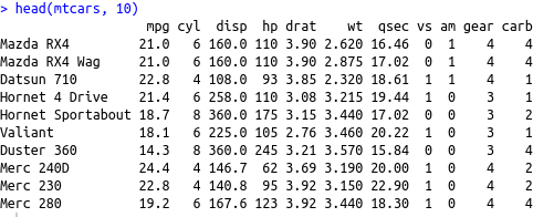
We can see that all the columns are numerical and hence, we can move forward with analysis. We’ll use the prcomp() function from the ‘stats’ package for conducting the PCA.
PCA with Covariance Matrix
First, we’ll conduct the PCA with the covariance matrix. For that, we set the scale option to false:
# Setting the scale=FALSE option will use the covariance matrix to get the PCs
cars.PC.cov = prcomp(mtcars[,-11], scale=FALSE) # sellecting the 11 columns by indexing mtcars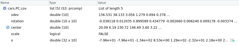
Here, cars.PC.cov is the result of the Principal Component Analysis on the mtcars data set using the covariance matrix. So, prcomp() returns five key measures: sdev, rotation, center, scale and x.
Let’s briefly go through all the measures here:
The center and scale provide the respective means and standard deviation of the variables that we used for normalization before implementing PCA.
sdev shows the standard deviation of principal components. In other words, sdev shows the square roots of the eigenvalues.
The rotation matrix contains the principal component loading. This is the most important result of the function. Each of the rotation matrix’s columns contains the principal component loading vector. We can represent the component loading as the correlation of a particular variable on the respective PC (principal component). It can assume both positive or negative. The higher the loading value, the higher the correlation. With the component loading information, you can easily interpret the PC’s key variable.
Matrix x has the principal component score vectors.
If you look at the prcomp function, you’ll see the ‘scale’ argument here is set to false as we specified in the input arguments.
Now, let’s look at the principal component loading vectors:
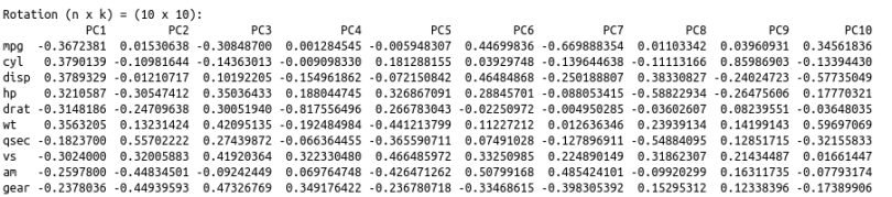
To help us interpret what we’re looking at here, let’s plot these results.
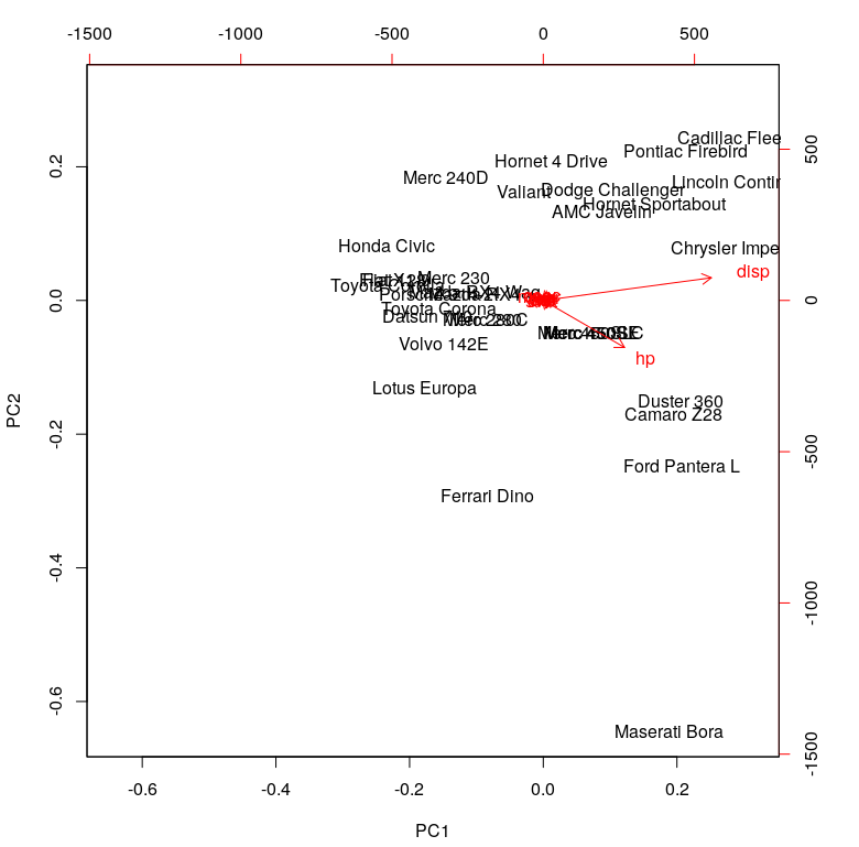
To read this chart, look at the extreme ends (top, down, left and right). The first principal component (on the left and right) correspond to the measure of ‘disp’ and ‘hp.’ The second principal component (PC2) does not seem to have a strong measurement.
We can finish this analysis with a summary of the PCA with the covariance matrix:
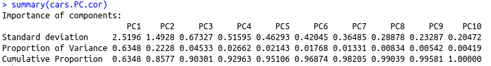
summary(cars.PC.cov)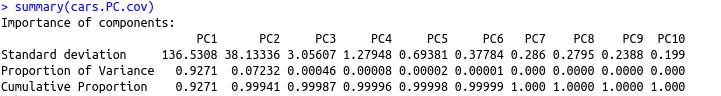
From this table, we see that PC1 made the maximum contribution to variation caused (~92.7%).All other principal components have progressively lower contribution.
In simpler terms, this means we can explain almost 93 percent of the variance in the data set using the first principal component with measures of ‘disp’ and ‘hp.’ This is in line with our observations from the rotation matrix and the plot above. As a result, we can’t draw many significant insights from the PCA on the basis of the covariance matrix.
PCA with Correlation Matrix
Now, let’s shift our focus to PCA with the correlation matrix. For this, all we need to do is set the scale argument to true.
# scale=TRUE performs the PCA using the correlation matrix
cars.PC.cor = prcomp(mtcars[,-11], scale=TRUE)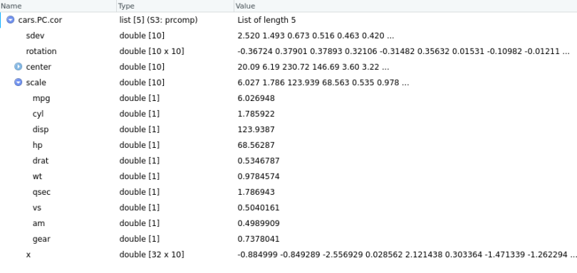
Using the same definitions for all the measures above, we now see that the scale measure has values corresponding to each variable. We can observe the rotation matrix in a similar way along with the plot.
# obtain the rootation matrix
cars.PC.cor$rotation
# obtain the biplot
biplot(cars.PC.cor)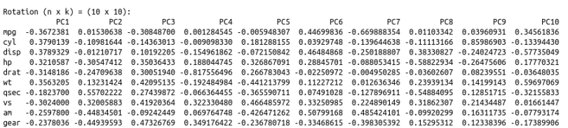
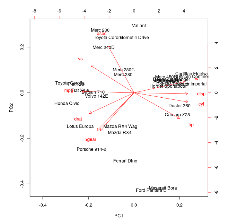
This plot looks more informative. It says variables like ‘disp,’ ‘cyl,’ ‘hp,’ ‘wt,’ ‘mpg,’ ‘drat’ and ‘vs’ contribute significantly to PC1 (first principal component). 'Meanwhile, ‘qsec,’ ‘gear’ and ‘am’ have a significant contribution to PC2. Let’s look at the summary of this analysis.
One significant change we see is the drop in the contribution of PC1 to the total variation. It dropped from 92.7 percent to 63.5 percent. On the other hand, the contribution of PC2 has increased from 7 percent to 22 percent. Furthermore, the component loading values show that the relationship between the variables in the data set is way more structured and distributed. We can see another significant difference if you look at the standard deviation values in both results above. The values from PCA while using the correlation matrix are closer to each other and more uniform as compared to the analysis using the covariance matrix.
The analysis with the correlation matrix definitely uncovers better structure in the data and relationships between variables. Using the above example we can conclude that the results differ significantly when one tries to define variable relationships using covariance vs. correlation. This in turn, affects the importance of the variables we compute for any further analyses. The selection of predictors and independent variables is one prominent application of such exercises.
Now, let’s look at another example to check if standardizing the data set before performing PCA actually gives us the same results. To showcase agility of implementation across technologies, I’ll execute this example in Python. We’ll consider the ‘iris’ data set.
from sklearn import datasets
import pandas as pd

# load iris dataset
iris = datasets.load_iris()
# Since this is a bunch, create a dataframe
iris_df=pd.DataFrame(iris.data)
iris_df['class']=iris.target

iris_df.columns=['sepal_len', 'sepal_wid', 'petal_len', 'petal_wid', 'class']
iris_df.dropna(how="all", inplace=True) # remove any empty lines

#selecting only first 4 columns as they are the independent(X) variable
# any kind of feature selection or correlation analysis should be first done on these
iris_X=iris_df.iloc[:,[0,1,2,3]]
Now we’ll standardize the data set using the inbuilt function.
from sklearn.preprocessing import StandardScale
# let us now standardize the dataset
iris_X_std = StandardScaler().fit_transform(iris_X)
I’ve now computed three matrices:
Covariance matrix on standardized data
Correlation matrix on standardized data
Correlation matrix on unstandardized data
# covariance matrix on standardized data
mean_vec = np.mean(iris_X_std, axis=0)
cov_matrix = (iris_X_std - mean_vec).T.dot((iris_X_std - mean_vec)) / (iris_X_std.shape[0]-1)
print('Covariance matrix \n%s' %cov_matrix)

# correlation matrix:
cor_matrix = np.corrcoef(iris_X_std.T)
print('Correlation matrix using standardized data\n%s' %cor_matrix)


cor_matrix2 = np.corrcoef(iris_X.T)
print('Correlation matrix using base unstandardized data \n%s' %cor_matrix2)
Let’s look at the results:
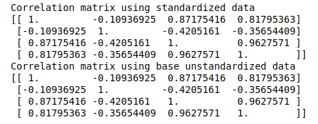
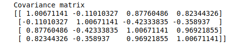
Here, it looks like the results are similar.
The similarities (fractional differences) reinforce our understanding that correlation matrix is just a scaled derivative of the covariance matrix. Any computation on these matrices should now yield the same or similar results.
To perform a PCA on these matrices from scratch, we’ll have to compute the eigenvectors and eigenvalues:
eig_vals1, eig_vecs1 = np.linalg.eig(cov_matrix)
print('Eigenvectors using covariance matrix \n%s' %eig_vecs1)
print('\nEigenvalues using covariance matrix \n%s' %eig_vals1)

eig_vals2, eig_vecs2 = np.linalg.eig(cor_matrix)
print('Eigenvectors using correlation matrix of standardized data \n%s' %eig_vecs2)
print('\nEigenvalues using correlation matrix of standardized data \n%s' %eig_vals2)

eig_vals3, eig_vecs3 = np.linalg.eig(cor_matrix2)
print('Eigenvectors using correlation matrix of unstandardized data \n%s' %eig_vecs3)
print('\nEigenvalues using correlation matrix of unstandardized data \n%s' %eig_vals3)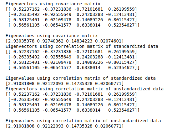
As expected, the results from all three relationship matrices are the same. We’ll now plot the explained variance charts from the eigenvalues we obtained:
# PLOTTING THE EXPLAINED VARIANCE CHARTS

##################################
#USING THE COVARIANCE MATRIX
##################################
tot = sum(eig_vals1)
explained_variance1 = [(i / tot)*100 for i in sorted(eig_vals1, reverse=True)]
cum_explained_variance1 = np.cumsum(explained_variance1)

trace3 = Bar(
        x=['PC %s' %i for i in range(1,5)],
        y=explained_variance1,
        showlegend=False)

trace4 = Scatter(
        x=['PC %s' %i for i in range(1,5)],
        y=cum_explained_variance1,
        name='cumulative explained variance')

data2 = Data([trace3, trace4])

layout2=Layout(
        yaxis=YAxis(title='Explained variance in percent'),
        title='Explained variance by different principal components using the covariance matrix')

fig2 = Figure(data=data2, layout=layout2)
py.iplot(fig2)

##################################
#USING CORRELATION MATRIX
##################################
tot = sum(eig_vals3)
explained_variance = [(i / tot)*100 for i in sorted(eig_vals3, reverse=True)]
cum_explained_variance = np.cumsum(explained_variance)

trace1 = Bar(
        x=['PC %s' %i for i in range(1,5)],
        y=explained_variance,
        showlegend=False)

trace2 = Scatter(
        x=['PC %s' %i for i in range(1,5)],
        y=cum_explained_variance,
        name='cumulative explained variance')

data = Data([trace1, trace2])

layout=Layout(
        yaxis=YAxis(title='Explained variance in percent'),
        title='Explained variance by different principal components using the correlation matrix')

fig = Figure(data=data, layout=layout)
py.iplot(fig)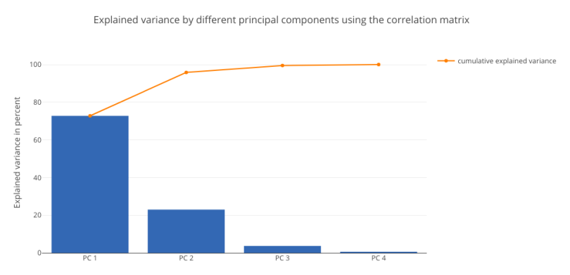

The charts resemble each other. Both the charts show that PC1 has the maximum contribution of around 71 percent. This analysis establishes the fact that standardizing the data set, then computing the covariance and correlation matrices will yield the same results.
We can use these strategies to apply the concept of variable relationships judiciously before using any predictive algorithm.